week 06 / 12
Understanding models trained on small tasks
Reverse engineer learned algorithms in models trained on small, controlled tasks.
companion notebook · ARENA 1.5.1, 1.5.2, and 1.5.4
new terms this week · 8
Representation concepts
- Superposition
- Representing more features than dimensions by packing sparse features into overlapping directions.
- Sparsity
- The property that most possible features are inactive for any given input.
- Polysemantic neuron
- A neuron that responds to multiple unrelated features.
Training dynamics
- Grokking
- A delayed transition where a model moves from memorization to real generalization long after fitting the training set.
- Progress measure
- A quantity computed during training that tracks the gradual formation of a mechanism, even while headline loss or accuracy is flat.
Spectral analysis
- Fourier basis
- A way to represent periodic patterns as sums of sine and cosine waves.
- FFT
- Fast Fourier transform: an efficient algorithm for computing a signal's discrete Fourier transform and revealing its frequency components.
Causal methods
- Restricted ablation
- An ablation that removes everything except a hypothesized subspace or mechanism.
This week covers three small models: a transformer that classifies balanced brackets, a transformer that adds numbers modulo 113, and a toy superposition model paired with a sparse autoencoder. Each provides unusually direct ground truth: the exact bracket-validity rule, the modular sum, or synthetic features chosen before training. A model can match every target while using a different internal method from the one we expected. Precisely specified targets and internal quantities let us make falsifiable claims about that method, a level of control that is rare when studying language models.
Week 6 notebooks
Compare three learned mechanisms
Work through the three notebooks:
- 1.5.1 Balanced Bracket Classifier: complete Section 1 “Bracket classifier,” Section 2 “Moving backwards,” and Section 3 “Understanding the total elevation circuit,” stopping after the total-elevation circuit summary.
- 1.5.2 Grokking & Modular Arithmetic: complete Section 1 “Periodicity & Fourier basis” and Section 2 “Circuit and Feature Analysis.”
- 1.5.4 Toy Models of Superposition & SAEs: complete Section 1 “TMS: Superposition in a Nonprivileged Basis” and Section 5 “Sparse Autoencoders in Toy Models.” Read only the introduction and brief conceptual material in Section 2.
Use a three-row comparison to organize your notes, one row per notebook. Record the target behavior, proposed mechanism, supporting measurement, intervention or control, and evidence limit. For 1.5.4, compare the SAE's learned feature directions and held-out activation patterns with the known toy-model features.
Stretch: Grokking (delayed generalization) Section 3 “Analysis During Training”; Superposition (overlapping feature directions) Sections 3–4; Balanced Brackets bonus and adversarial examples; OthelloGPT; or one Monthly Algorithmic Problem.
Slides: Understanding models trained on small tasks
Why small tasks help
Small tasks give us a known function to compare against. For balanced brackets, a string is invalid as soon as a prefix contains more closing brackets than opening brackets. The superposition experiment also tells us which input features exist and how often each fires because we chose them.
Even with a known rule, accuracy only tells us how the model behaved on the examples tested. A mechanistic explanation needs to connect four things:
- the mathematical function the model should compute;
- the internal quantities it represents while computing that function;
- the components that transform and move those quantities; and
- an intervention whose effect matches the explanation's prediction.
Three measurements help identify a possible mechanism. Weight spectra reveal dominant patterns in learned weights. Direct logit attribution estimates a component's direct contribution to a chosen output logit. Activation fits compare observed activations with a hypothesized quantity. However, all three are correlational.
Last week, we were introduced to activation patching. This technique replaces an internal activation with one from another input and measures the output change. Removing a proposed computation and observing the predicted degradation supports necessity. Retaining only that computation and observing preserved performance supports approximate sufficiency. Patching an internal value and observing the predicted logit change supplies local causal evidence. It is important to remember that no one measurement proves that the proposed circuit is the model's only route to the answer. We begin with balanced brackets because its target rule is simple enough to write by hand, even though the transformer's implementation spreads the work across attention heads and MLPs.
Balanced bracket classifier
The usual way to check a bracket string is to keep a running_balance. Start at zero, add one for (, and subtract one for ). For (()()), the balance is 1, 2, 1, 2, 1, 0. It never becomes negative and ends at zero, so the string is balanced.
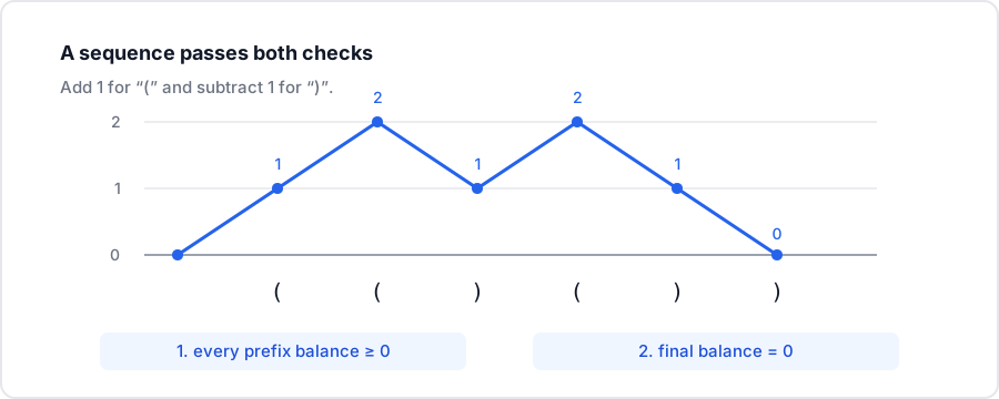
The two invalid strings in the code separate the ways this can fail. )(()() has balances -1, 0, 1, 0, 1, 0: it ends at zero but reaches -1 immediately. (()(() has balances 1, 2, 1, 2, 3, 2: it never goes negative but ends at 2.
The final balance is the total elevation. A left-to-right prefix balance gives the mathematical validity rule. The source plot uses a second diagnostic based on right-to-left suffix elevations: it maps ( to 1 and ) to -1, reverses the sequence, and checks whether any cumulative sum is positive. This suffix diagnostic matches the negative-prefix check when total elevation is zero. The two can differ when the counts do not match. (()(() shows the difference. Its reversed cumulative sums are -1, 0, 1, 0, 1, 2, so it fails the suffix check even though no left-to-right prefix goes negative. It also fails total elevation.
total_elevation_failuremeans the final balance is nonzero.prefix_negativemeans a left-to-right prefix balance goes below zero.negative_failureis the suffix-based diagnostic used to color the source plot. The plot labels it suffix failure.
The model was trained only to predict balanced or unbalanced. The code below derives that binary label and the two diagnostics used in the analysis.
Edit a sequence, then run it on the course CPU.
def diagnose(sequence):
    balance = 0
    lowest = 0
    for bracket in sequence:
        balance += 1 if bracket == "(" else -1
        lowest = min(lowest, balance)
    total_elevation_failure = balance != 0
    prefix_negative = lowest < 0

    suffix_elevation = 0
    negative_failure = False
    for bracket in reversed(sequence):
        suffix_elevation += 1 if bracket == "(" else -1
        negative_failure |= suffix_elevation > 0

    balanced = not total_elevation_failure and not prefix_negative
    return total_elevation_failure, prefix_negative, negative_failure, balanced

for sequence in ["(()())", ")(()()", "(()(()"]:
    total, prefix_negative, negative_failure, balanced = diagnose(sequence)
    print(
        f"{sequence:6} total_failure={str(total):5} "
        f"prefix_negative={str(prefix_negative):5} "
        f"negative_failure={str(negative_failure):5} balanced={balanced}"
    )
# (()()) total_failure=False prefix_negative=False negative_failure=False balanced=True
# )(()() total_failure=False prefix_negative=True  negative_failure=True  balanced=False
# (()(() total_failure=True  prefix_negative=False negative_failure=True  balanced=False
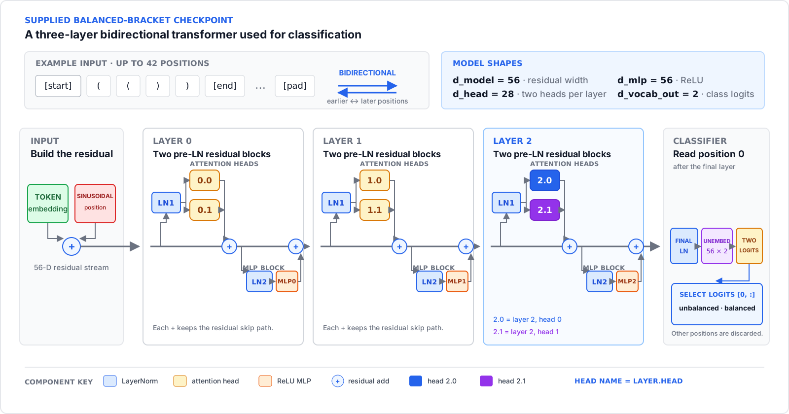
The classifier is loaded from a checkpoint, a saved copy of its learned weights from a particular point in training. It has three pre-LayerNorm transformer layers, meaning normalization occurs before each sublayer. The residual stream is the shared vector representation updated by those sublayers. Each layer has two bidirectional attention heads and an MLP whose ReLU activation keeps positive neuron inputs and sets negative ones to zero. A residual connection adds each sublayer's output back to the shared representation. Position 0 holds the start token from which this classifier reads its prediction. The final unembedding maps the residual representation there to the balanced and unbalanced logits. We write heads as layer.head, so head 2.0 means head 0 in layer 2.
Scroll sideways to inspect the full model.
Interactive model
Inspect the bracket classifier
Choose or generate a bracket sequence, then inspect its bidirectional attention, layer activations, logits, and prediction. The explainer runs the supplied ARENA checkpoint.
Direct logit attribution estimates each head's direct contribution to the unbalanced-minus-balanced logit difference. In the supplied checkpoint, head 2.0 contributes most for nonzero total elevation, while head 2.1 contributes most for suffix failure. Their roles overlap, so this is a division of labor rather than a clean one-head-per-rule split.
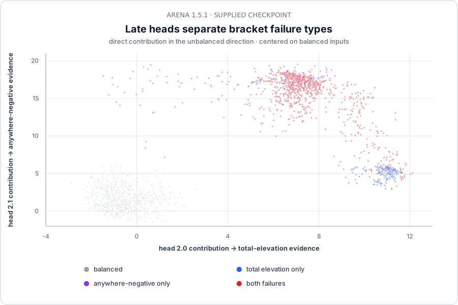
Each axis is that head's centered direct contribution along the unbalanced-minus-balanced logit direction, for 3,604 strings. Balanced inputs sit near the origin. The source run drops sequences that start with ). Source plot.
Total-elevation failures move mainly along the head 2.0 axis, while suffix failures move mainly along the head 2.1 axis. Strings that fail both diagnostics receive a push from both heads. The colors come from the hand-written rule above instead of a pattern fitted to the model.
Watch: trace one bracket prediction through the circuit

The walkthrough traces the start token, opens one attention calculation, follows the value written back to the start position, and ends at the unbalanced prediction. Use the live explainer above to change the sequence.
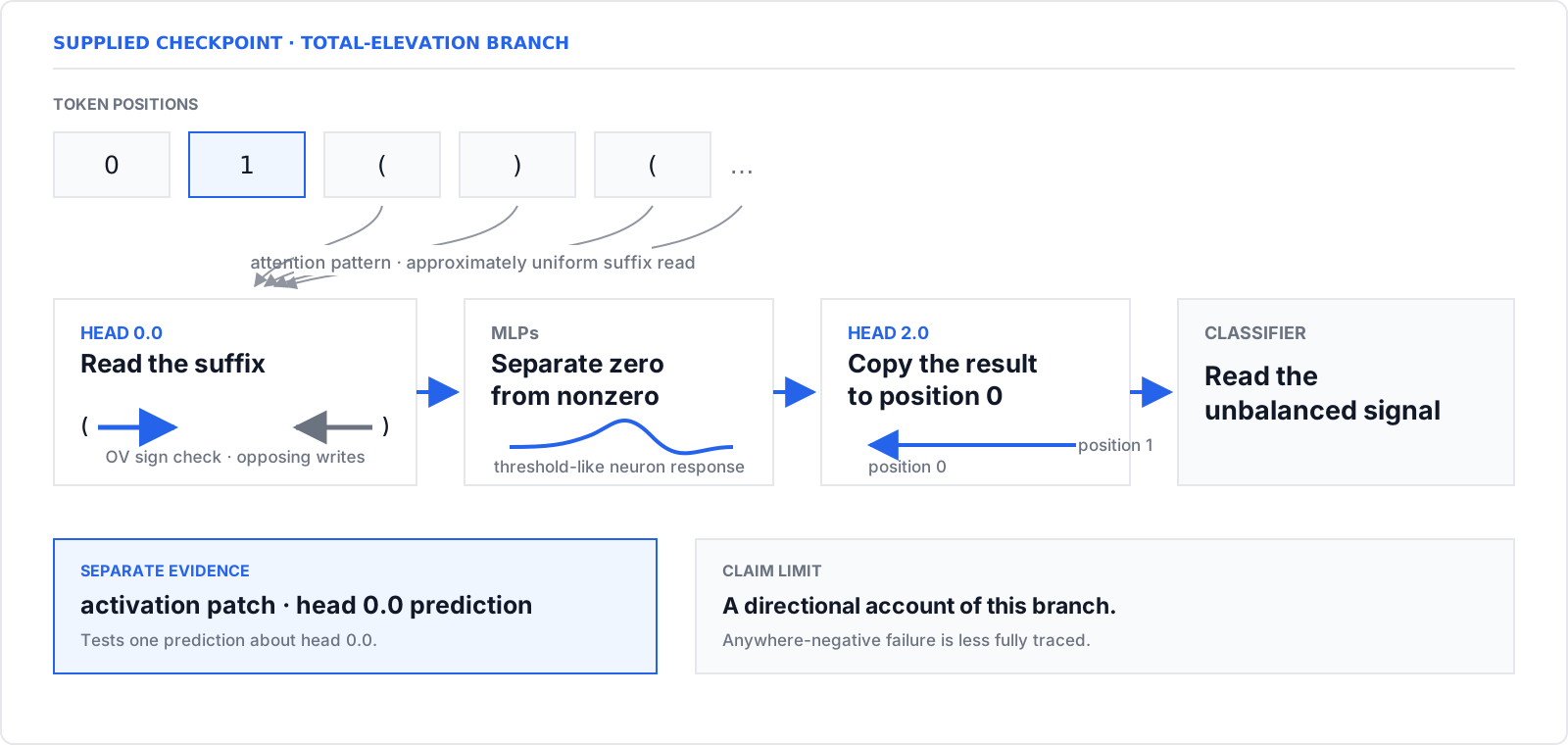
An attention head's OV map determines what information an attended source writes to the residual stream. The total-elevation branch has a direct source-to-classifier sequence. Head 0.0 reads roughly uniformly from positions in the relevant suffix. Its OV map writes ( and ) in opposing directions. Residual addition combines those writes at position 1 into a continuous tally. MLP neurons produce a threshold-like distinction between zero and nonzero elevation. Head 2.0 copies that signal to position 0. The unembedding turns the copied signal into evidence for the unbalanced class.
Each analysis tool supplies a different piece of evidence:
- Direct logit attribution identifies components whose outputs align with the unbalanced-minus-balanced logit direction.
- Attention patterns identify the source positions a head reads from, but not the content it writes.
- A head's OV map identifies that written content. Opposite writes for
(and)provide the signed contributions needed for a tally. - Neuron plots associate MLP activity with elevation, but do not establish that those neurons are required.
- Activation patching is a causal check to perform: patch head 0.0 and compare the logit change with the circuit's prediction. No patching outcome is reported here.
Together, these measurements support the proposed path, but they do not make it exact. A single residual direction can miss indirect routes. LayerNorm is nonlinear, so treating the path as a chain of matrix multiplications requires a local linear approximation. That approximation can hide a real path or make a weak one look stronger than it is. The evidence is stronger for the total-elevation branch than for the suffix-based negative_failure branch.
Grokking and modular arithmetic
Grokking is a delayed transition from memorizing the training set to generalizing beyond it. Here we study a one-layer transformer trained to predict (x + y) mod 113 from the tokens [x, y, =]. For example, 100 + 50 = 150, and 150 mod 113 = 37, so the correct output is 37. The model has four attention heads, a 128-dimensional residual stream, and a 512-dimensional MLP. This analysis describes the algorithm in the supplied final checkpoint, not when or why the grokking transition happened.
Modular addition wraps after 113, so residues can be represented as points on a circle. The Fourier basis describes functions on that circle with sine and cosine waves. For a frequency index k, define ω = 2πk / 113. A residue x maps to phase ωx, represented by sin(ωx) and cos(ωx).
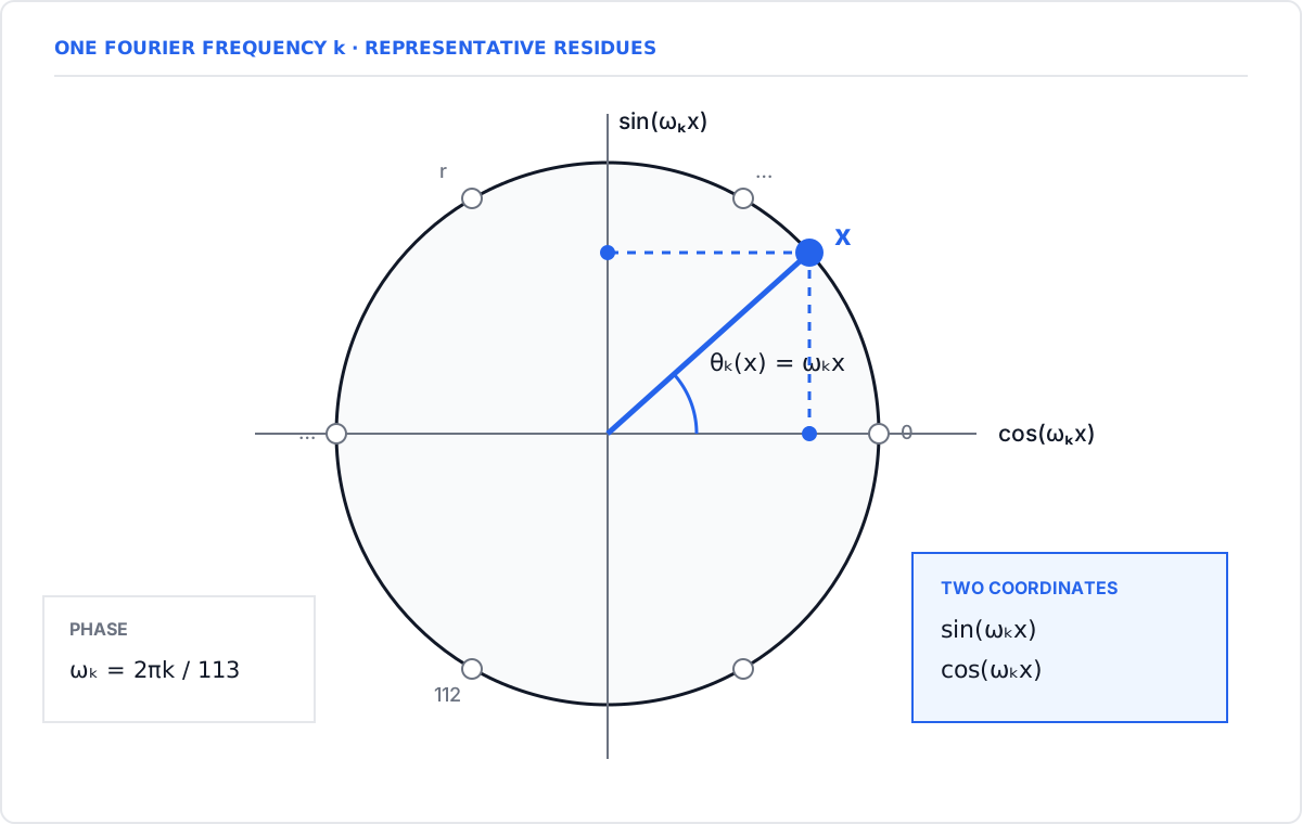
Transforming the model's embeddings, activations, and effective weights (the composed linear maps between components) into that basis concentrates most of their energy at a handful of key frequencies. That concentration supports periodic organization rather than pure pairwise memorization. Memorized contributions can still remain. A sharp peak identifies a useful coordinate system. It does not show how attention combines x and y, how the MLP forms angle-addition terms, or how the unembedding scores z.
At one frequency, let a = ωx and b = ωy. The embeddings supply sin(a), cos(a), sin(b), and cos(b), and attention brings both operands together. The ReLU MLP approximates the products in the angle-addition identities:
cos(a + b) = cos(a)cos(b) - sin(a)sin(b)
sin(a + b) = sin(a)cos(b) + cos(a)sin(b)
These terms represent the phase of the sum. Comparing that phase with candidate z gives cos(ω(x + y - z)). For x = 100, y = 50, and z = 37, the difference is 113. At every retained integer frequency, the contribution is cos(2πk) = 1. Incorrect candidates generally do not align across the retained frequencies, so their contributions tend to cancel.
Each of the 512 MLP neurons is fit to candidate Fourier terms across frequencies. The plot records its best-fitting frequency and its explained fraction, the fraction of activation variance accounted for by the best Fourier fit. Neurons with explained fraction at or above 0.85 cluster around five frequencies. The fit supports Fourier structure in MLP activations. Attention also contributes operand-dependent products, so the MLP is not the whole quadratic step.
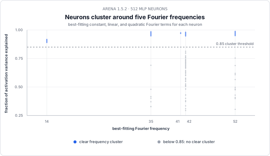
All 512 MLP neurons are plotted by best-fitting frequency (x) and explained fraction (y). Blue marks the clear cluster at or above 0.85; gray marks neurons below the threshold at their best-fitting real frequency. Reproduced from the ARENA 1.5.2 notebook output.
The code below uses the five frequency clusters in the MLP neuron plot to score all 113 possible answers:
Change x, y, or the frequencies, then run it on the course CPU.
import math

p = 113
x, y = 100, 50
frequencies = [14, 35, 41, 42, 52]
logits = [
    sum(math.cos(2 * math.pi * k * (x + y - z) / p) for k in frequencies)
    for z in range(p)
]
ranking = sorted(range(p), key=logits.__getitem__, reverse=True)
prediction = ranking[0]
print("prediction:", prediction)
print("target:    ", (x + y) % p)
print("margin:    ", round(logits[ranking[0]] - logits[ranking[1]], 3))
# prediction: 37
# target:     37
# margin:     2.41
The five-frequency scorer predicts 37 with a clear margin. This checks the proposed output rule, but does not show that the trained model performs the calculation. Model-specific measurements connect the rule to the model's weights, activations, and behavior under restricted computation. Projected logits keep the component in a chosen Fourier subspace. Restricted computation retains only selected internal directions or neurons and measures performance.
Compare three intervention conditions:
- Keep the key frequencies to test approximate sufficiency.
- Remove the key frequencies to test necessity.
- Keep a random same-sized set as a matched control.
Report accuracy or loss together with the fraction of the model retained. Projecting only the logits into a hand-picked subspace is a weaker test because the rest of the model still performs its full computation before that projection. No restricted-model outcome is reported here, so necessity and approximate sufficiency remain measurements to perform.
A later checkpoint replay can track progress measures while the train/test split stays fixed: excluded loss is loss after removing the key-frequency contribution; embedding singular values show how concentrated or low-rank the embedding matrix is; Fourier structure measures concentration in key frequencies; commutativity measures sensitivity to swapping x and y; and weight norms measure the magnitudes of selected weights. A flat test-loss curve does not imply that the internals have stopped changing. A changing internal metric does not by itself identify the cause of the later transition. Compare seeds and regularization settings before making a training-dynamics claim.
Balanced brackets and modular addition connect transformer behavior to a learned algorithm. Superposition shifts the analysis from algorithms to features in a hidden representation. Week 4 treated SAE latent meanings as hypotheses in language-model activations. Here synthetic data supplies known ground-truth features, so SAE recovery can be measured directly.
Superposition and sparse autoencoders
The features are defined before training. Each input coordinate has known importance and activation probability. A small model compresses those features into fewer hidden dimensions and reconstructs them. The chosen dictionary permits ground-truth comparison instead of relying on examples that merely look meaningful.
Suppose we need to place five feature directions in a two-dimensional hidden space. They cannot all be orthogonal, so some directions must overlap. If most features activate on every input, those overlaps cause frequent collisions. The model tends to reserve dimensions for the most important features and drop the rest. If only a few features activate at once, the same overlaps cause fewer collisions, allowing the model to pack more feature directions into the space. This overlapping representation is superposition, the idea introduced in week 4 to explain why raw activation coordinates can be hard to read. A feature-direction Gram matrix contains pairwise dot products between directions; its off-diagonal entries measure overlap.
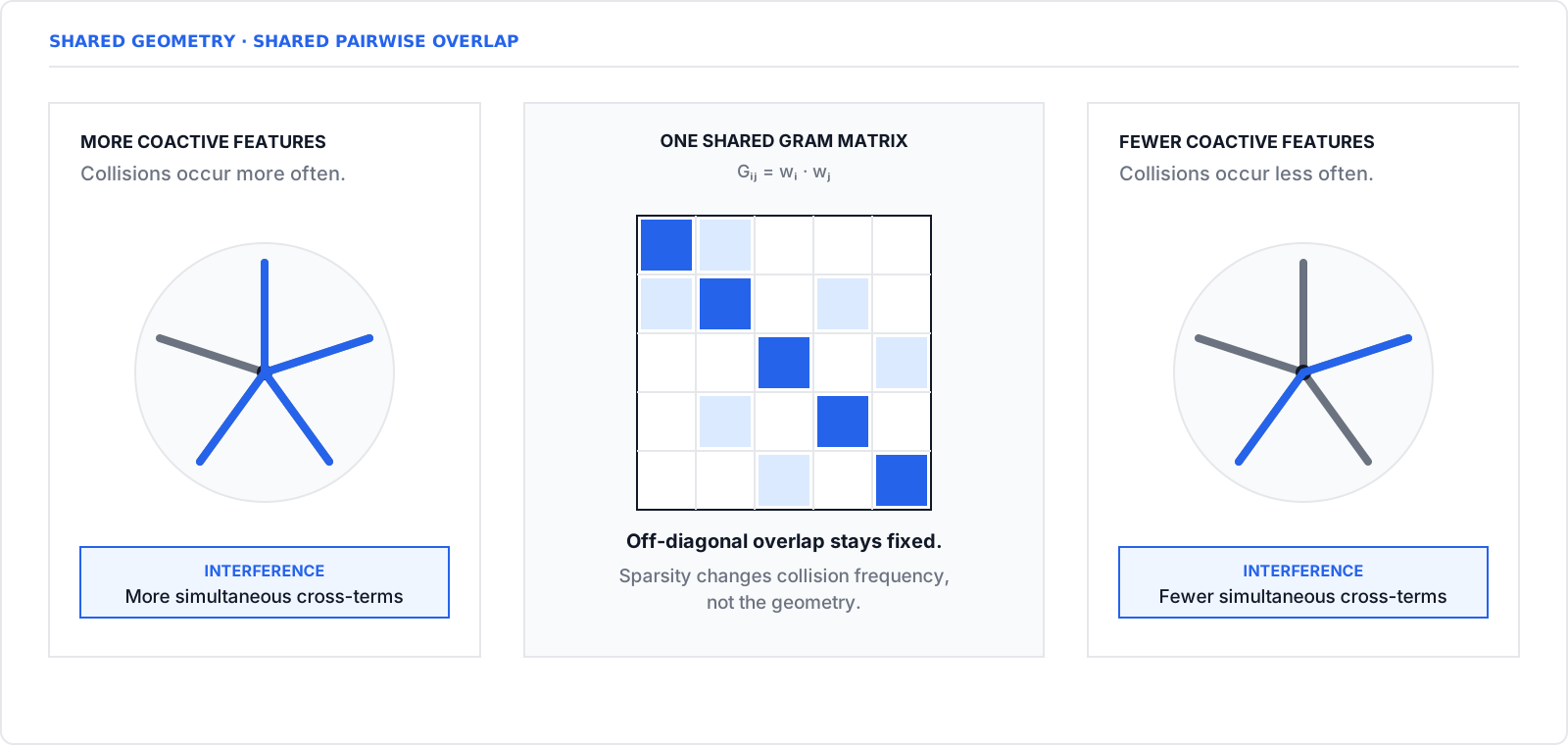
The code below computes that interference directly. With one active feature, two small positive projections survive ReLU. Activating two overlapping features at once produces a larger reconstruction error.
Change the active feature pair, then run it on the course CPU.
import math

directions = [
    (
        math.cos(math.pi / 2 + 2 * math.pi * i / 5),
        math.sin(math.pi / 2 + 2 * math.pi * i / 5),
    )
    for i in range(5)
]

def dot(a, b):
    return sum(ai * bi for ai, bi in zip(a, b))

overlaps = [[dot(a, b) for b in directions] for a in directions]

for active in ([0], [0, 2]):
    x = [float(i in active) for i in range(5)]
    raw = [
        sum(overlaps[i][j] * x[j] for j in range(5))
        for i in range(5)
    ]
    reconstruction = [max(0.0, value) for value in raw]
    mse = sum((actual - predicted) ** 2 for actual, predicted in zip(x, reconstruction)) / 5
    print(
        f"active={active}: reconstruction="
        f"{[round(value, 2) for value in reconstruction]}, mse={mse:.3f}"
    )
# active=[0]: reconstruction=[1.0, 0.31, 0.0, 0.0, 0.31], mse=0.038
# active=[0, 2]: reconstruction=[0.19, 0.62, 0.19, 0.0, 0.0], mse=0.338
The fixed geometry explains why sparse inputs can tolerate overlaps that cause trouble for dense inputs. Training the toy model on sparse and dense data tests the predicted solutions: dedicated dimensions for dense features, and overlapping directions for sparse ones. The directions in this calculation are fixed rather than learned, so it illustrates the geometric pressure rather than a training result.
The toy model maps a sparse vector of known input features into a compressed activation, where feature directions overlap. A sparse autoencoder is a second model. It encodes that activation into sparse latents, one learned coordinate each. Every latent has a decoder direction that maps it back into the reconstructed activation. Reconstruction loss rewards preserving the compressed activation, while the sparsity penalty discourages many latents from firing at once. Because the true hidden-space directions are known, each learned decoder direction can be compared directly with the feature direction that generated the data.
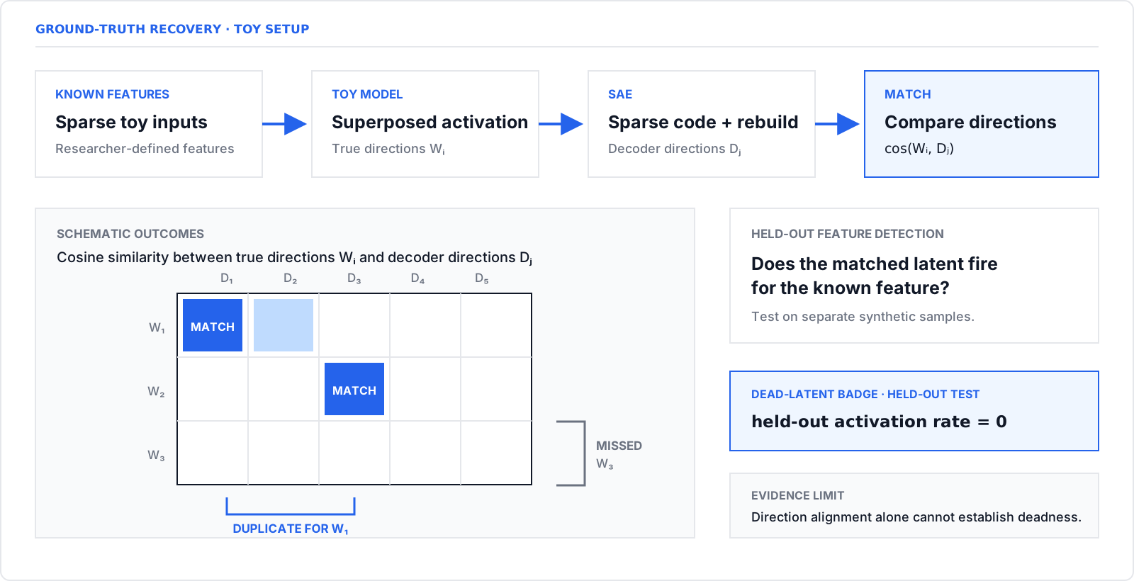
Low reconstruction loss is not enough. Cosine similarity measures directional alignment: 1 means the same direction, 0 means orthogonal, and -1 means opposite. Evaluate recovery with checks that establish different facts:
- Match decoder directions to true feature directions with cosine similarity. This establishes geometric alignment, but not feature detection.
- Compare held-out activations when each feature is present and absent. Firing for present examples and staying quiet for absent examples establishes selective detection.
- Enforce and report one-to-one coverage between latents and true features. This reveals duplicate matches and missed features.
- Measure each latent's held-out activation rate. A zero rate flags the latent as dead on that held-out set; report the sample size.
- Report reconstruction loss as reconstructability only. Distributed, duplicated, or dense codes can also reconstruct well.
These are recovery criteria. No trained-SAE recovery result is reported on this page. Compare SAEs at matched width, the number of latents, and matched sparsity pressure, the strength of the penalty on latent activity, because a wider or denser code can improve reconstruction without producing a cleaner decomposition. Successful toy recovery shows that an SAE can recover known features under these assumptions. It does not show that language-model activations follow the same feature model or that every learned latent has one stable meaning.
In a purely linear encoder-decoder, rotating the encoder representation and applying the inverse rotation in the decoder preserves the output, so no coordinate axis is special. Coordinatewise ReLU breaks this symmetry because rotation changes which individual coordinates pass the threshold. The neuron axes can then become a preferred basis.
Reporting results
For each result, record the model checkpoint, random seed, metric, and control so someone else can interpret the comparison. Keep the plot or table that supports each row of your notes. The superposition exercises batch several independent toy models and examples in one tensor: instances indexes independently trained toy models, batch indexes input examples, feature indexes known input coordinates, and hidden indexes the compressed representation. Mixing these axes averages different experimental quantities rather than repeated measurements of the same quantity. Exact plots and metrics depend on the supplied checkpoint, notebook version, optimization seed, and completed section. Report observed values rather than copying expected numbers from another run.
Stretch work
OthelloGPT predicts legal Othello moves from a sequence of prior moves. Linear probes measure how well board properties can be decoded from its activations. Interventions along those probe directions, including with activation patching, measure the effect of changing the decoded board state on legal-move predictions. Probe accuracy establishes readability. The intervention supplies evidence that the model uses the representation. Keep conclusions tied to board state, this model, and these interventions. Readability plus a local causal effect does not establish a general world model.
Monthly Algorithmic Problems offer shorter group investigations. Choose one behavior, define a metric before opening model internals, and end with a falsifiable circuit claim. A small task is useful because it permits tighter tests, not because every result transfers to a language model.
Further reading
- The ARENA toy-model overview explains the goals and limits of this chapter.
- Nanda et al., Progress measures for grokking via mechanistic interpretability, gives the Fourier-circuit and training-dynamics analysis used here.
- Power et al., Grokking: Generalization Beyond Overfitting on Small Algorithmic Datasets, introduced the delayed-generalization result.
- Elhage et al., Toy Models of Superposition, motivates the synthetic feature model and its geometric predictions.
- Li et al., Emergent World Representations: Exploring a Sequence Model Trained on a Synthetic Task, introduces the OthelloGPT model and its board-state probing results.
this week's practice
core
- Complete 1.5.1 Sections 1–2 and Section 3 through the total-elevation circuit summary
- Complete 1.5.2 Sections 1–2: Periodicity & Fourier basis and Circuit and Feature Analysis
- Complete 1.5.4 Sections 1 and 5, plus the introduction and brief conceptual material in Section 2
- Submit one three-row comparison with a target behavior, mechanism, measurement, intervention or control, and evidence limit in each row
stretch
- Complete 1.5.2 Section 3 Analysis During Training
- Complete 1.5.4 Sections 3–4
- Try the 1.5.1 bonus and adversarial examples
- Complete 1.5.3 OthelloGPT
- Try a Monthly Algorithmic Problem