week 04 / 12
Probes, steering vectors, and SAEs
Read activations with probes, edit them with steering vectors, and decompose them with SAEs.
companion notebook · ARENA 1.3.3
new terms this week · 18
Representation concepts
- Feature
- A property of the data or the computation that researchers may want to track. Features exist in the data distribution whether or not an SAE finds them.
SAE methods
- Sparse autoencoder (SAE)
- A model trained to reconstruct activations using a sparse, wider latent representation.
- SAE latent
- One learned coordinate of an SAE: an encoder direction that decides when it fires, and a decoder direction it writes back. A candidate representation of one or more features, not a feature by definition.
- L0
- The average number of SAE latents active on a token. The standard sparsity measure for an SAE.
Tools
- sae_lens
- An open-source library for loading, training, and evaluating sparse autoencoders on model activations.
- Neuronpedia
- A public browser for inspecting model neurons and SAE features.
- nnsight
- A tracing and intervention library for reading and editing model internals, including remotely hosted models.
Feature analysis
- Feature dashboard
- A report showing examples, stats, and effects for one SAE latent or neuron.
Probing
- Linear probe
- A simple linear classifier trained on activations to test whether information is linearly readable.
- Mass-mean probe
- A linear probe whose direction is the difference between the mean activation for each of two labeled classes, computed in closed form rather than fitted by optimization. It scores raw activations with no intercept.
- Logistic regression
- A linear classifier that fits a weight vector by optimization, then maps its score to a class probability with the logistic function. The probes fitted this week standardize activations first and fit no intercept.
- Truth direction
- A direction in activation space associated with true versus false statements.
Data analysis
- PCA
- Principal component analysis: a way to project high-dimensional activations onto high-variance directions.
Experimental design
- Confound
- A variable correlated with the label that can create an apparent effect without representing the property the experiment aims to measure.
- Contrastive pair
- Two inputs matched except for a target property; subtracting their activations estimates a direction associated with that property.
Steering
- Steering vector
- A vector added to an activation to push model behavior in a chosen direction.
- Function vector
- An activation direction that appears to encode a task such as antonym generation.
- Activation addition
- An intervention that adds a chosen vector to a model activation during a forward pass to steer subsequent behavior.
Week 4 assignment
Test a latent in an SAE reconstruction
The probe and steering sections show what each method can establish; notebooks 1.3.1 and 1.3.2 are optional. Required work covers 1.3.3 and the layer-9 experiment.
- See why held-out probe accuracy does not prove the model uses that property. For steering, note how the baseline and coefficient sweep support a causal claim.
- Study the assigned latent on Neuronpedia and write a description a counterexample could disprove.
- Complete assigned 1.3.3 sections under Notebook session.
- Run the original model, then replace layer 9 with the full SAE reconstruction.
- Repeat after setting that latent to zero.
Use the full SAE reconstruction as the control. Comparing ablation only with the original model confounds latent removal with reconstruction error.
Before the run, predict the metric effect from Neuronpedia evidence. Compare your prediction with the result, limiting the conclusion to tested prompts and intervention.
Slides on probes, steering vectors, and SAEs
Video on probes, steering vectors, and SAEs
Open the video in a new tab if the embedded player does not load.
Three methods for studying model activations
Each method studies a different aspect of intermediate model activations. The table compares how they work and what their results can show.
| What it does | What it can tell you | What it cannot show by itself | |
|---|---|---|---|
| Probe | Fits a linear predictor to labelled activations | Whether held-out labels are linearly predictable at the tested layer | Whether the model relies on that property when producing its output |
| Steering | Edits an activation and reruns the model | How the chosen edit changes the measured behavior | Whether the result holds under another setup or prompt set |
| SAE | Encodes an activation with sparse latents, then reconstructs it | How well the sparse code preserves the activation | What a latent represents or whether it affects model behavior |
Keep each conclusion within the tested setup. Results may change with new data or a different intervention. Check counterexamples and alternative explanations before assigning a semantic label; broader claims need additional evidence.
Linear probes
A linear probe uses labelled activations to test whether a property can be predicted from them using a linear model. There are several ways to build one. One example is a mass-mean probe, which bases its predictions on the difference between the average positive and negative activations. Another is logistic regression, which learns a regularized linear classifier from the labelled activations.
The playground below shows how a mass-mean probe's direction changes when the labelled examples change.
toy playground · not a real activation
The direction depends on the labels
Eight points stand in for activations in two dimensions. Flip their True/False labels to change the mass-mean direction w = μ(true) − μ(false). The arrow starts at the midpoint of the class means as a visual anchor. That anchor has no role in probe scoring.
After fitting a probe, you can evaluate it on labelled examples that were not used to build it. Held-out accuracy measures how often the probe predicts these new labels correctly. A high score is evidence that the property can be predicted from activations at the tested layer for this dataset. It does not show that the model relies on the property when producing an answer, and the probe may have found an unrelated pattern in the data.
Function vectors
Last week, we saw one form of in-context computation: the model reused a token pattern from earlier in the prompt. Here, demonstrations of antonyms specify a different in-context task and can leave a task-encoding hidden state in the residual stream:
Antonym task · few-shot prompt
Q: hot A: cold Q: yes A: no Q: in A: out Q: up A:
A function vector tries to isolate that task signal in a small set of attention heads. To build one:
- Create clean prompts like the one above and corrupted versions with shuffled answers, so the demonstrations no longer show the task.
- For each attention head, average its output at the final prompt token across the clean prompts for one task. This task-conditioned mean is the value you patch.
- Patch one head's mean output into the corrupted runs at the final token and measure how much it restores the correct answer. This is the head's causal indirect effect.
- Average each head's indirect effect across many tasks and keep the heads with the largest average.
- Sum those heads' task-conditioned mean outputs into a single function vector for the task.
- Add the function vector to the residual stream at the final token of a prompt with no demonstrations and test whether the model performs the task.
Todd et al. (2023) select heads using effects aggregated across many tasks. A demonstration that selects heads from the antonym task alone is an adaptation of their method.
The playground below compares an unsteered completion with possible outputs at several vector strengths.
conceptual sweep · authored text, not model data
Compare outputs across steering strengths
Select a checkpoint to compare one possible edited completion with the same prompt at α = 0.
h add α·v edited state h′ completion h′ = h + α·v
These α values are schematic checkpoints, not a calibrated scale that transfers between models or steering setups.
Unsteered reference · α = 0
up
- Target task shown
- no
- Output quality
- fluent
Selected checkpoint · α = 0
up
- Target task shown
- no
- Output quality
- fluent
This is the unsteered reference condition.
Use the same prompts without the vector as a baseline. Then try several coefficients above and below zero, measuring task performance and output quality at each value. A reliable change shows that this intervention affected behavior in the tested setup. It does not prove that the vector uniquely represents the task or that the result extends to another layer or prompt set.
Sparse autoencoders
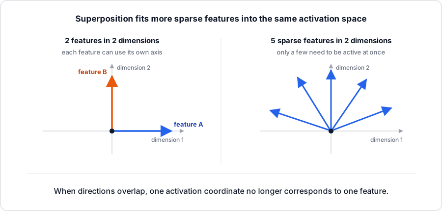
An activation may carry more features than it has orthogonal dimensions. When those features are sparse, a model can pack them into overlapping directions through superposition. This increases capacity, but it also makes individual neurons and activation dimensions harder to interpret.
A sparse autoencoder encodes an activation as a wider latent vector with only a few nonzero entries. The decoder uses those active latents to reconstruct .
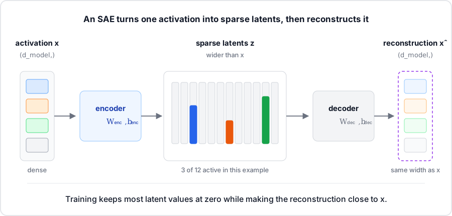
We use feature for a property of the data or computation and latent for one coordinate learned by the SAE. The mapping need not be one-to-one. A semantic label is a hypothesis to test.
The exact equations depend on the SAE architecture. The required gpt2-small-res-jb SAE uses ReLU and subtracts the decoder bias before encoding:
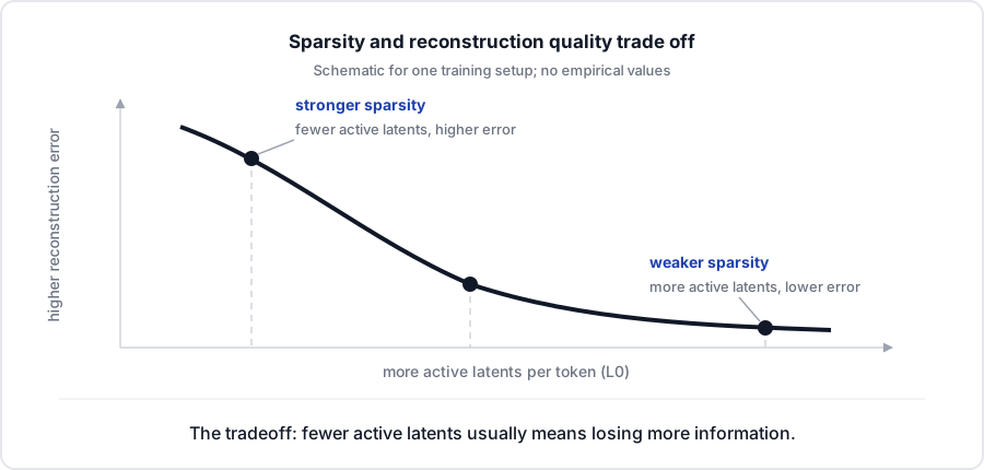
SAEs balance sparsity against reconstruction quality. Strong sparsity pressure makes fewer latents fire, which may make the representation easier to inspect but can discard information. Relaxing that pressure usually improves reconstruction and produces a denser code. Compare sparsity and reconstruction only within the same training setup. Other SAE architectures use different activation and sparsity rules, so check the loaded architecture before reusing these equations.
Investigate one SAE latent in Neuronpedia
This exercise uses an SAE trained on GPT-2 Small’s layer-9 residual stream. Open latent 21474 in Neuronpedia and begin with these views:
- Inspect the top activating examples to find contexts and tokens where the latent fires most strongly.
- Use the activation distribution to see how often it fires and at what strength.
- Check boosted and suppressed tokens to see which outputs align with the decoder direction after unembedding.
Other panels can add context. Read the autointerp label only after writing your own hypothesis.
Neuronpedia
GPT-2 Small, 9-res-jb, latent 21474
Watch: tour latent 21474 on Neuronpedia

Write your hypothesis as “Latent 21474 activates for ___ more than ___.” Record two examples that support it. Next, change only the suspected property in a minimal pair and look for a likely counterexample. Save the exact prompts and activations alongside the model name, SAE release, hook point, and latent ID.
Test a latent with ablation
Choose a fixed set of prompts and define a metric for the behavior you want to test before running the model. Then record these conditions:
- Run the original model without an SAE.
- Replace the layer-9 activation with the full SAE reconstruction.
- Repeat the reconstruction after setting latent 21474 to zero.
The 1.3.3 notebook introduces SAELens hooks at several layers. The example below fixes the hook at layer 9 and scores each prompt with the total next-token probability of five Star Wars names: a softmax over the full vocabulary, summed over the five target token IDs. A higher value means the model puts more probability on those names. Adding the same constant to every logit leaves this probability unchanged, while each raw target logit would rise. All three conditions use this metric. Run the example, then adapt its prompts and metric to test your hypothesis about the latent.
import torch as t
import warnings
from functools import partial
from sae_lens import SAE, HookedSAETransformer

t.set_grad_enabled(False)
device = "cuda" if t.cuda.is_available() else "cpu"
with warnings.catch_warnings():
    warnings.filterwarnings(
        "ignore",
        message=r"\s*This SAE has non-empty model_from_pretrained_kwargs\.",
    )
    sae = SAE.from_pretrained(
        release="gpt2-small-res-jb",
        sae_id="blocks.9.hook_resid_pre",
        device=device,
    )
model = HookedSAETransformer.from_pretrained_no_processing(
    "gpt2-small",
    device=device,
    **sae.cfg.metadata.model_from_pretrained_kwargs,
)
sae.use_error_term = False  # replace model activations with SAE reconstructions
hook_name = sae.cfg.metadata.hook_name
latent_idx = 21474
latent_hook = f"{hook_name}.hook_sae_acts_post"

prompts = [
    "Luke trained as a Jedi",
    "Luke trained as a wizard",
    "We cooked a simple soup",
]
tokens = model.to_tokens(prompts, padding_side="left")
target_tokens = [" Skywalker", " Vader", " Kenobi", " Solo", " Leia"]
target_ids = t.tensor(
    [model.to_single_token(token) for token in target_tokens],
    device=device,
)

def star_wars_score(logits):
    # Softmax over the full vocabulary, then sum the probability of the target names.
    probs = logits[:, -1, :].softmax(dim=-1)
    return probs[:, target_ids].sum(dim=-1)

original_logits = model(tokens, return_type="logits")
# Control: a uniform shift of every logit leaves the score unchanged.
t.testing.assert_close(star_wars_score(original_logits + 5.0), star_wars_score(original_logits))
reconstruction_logits, cache = model.run_with_cache_with_saes(
    tokens,
    saes=[sae],
    names_filter=[latent_hook],
    return_type="logits",
)

def ablate_latent(sae_acts, hook, latent_idx):
    sae_acts = sae_acts.clone()
    sae_acts[..., latent_idx] = 0.0
    return sae_acts

ablation_logits = model.run_with_hooks_with_saes(
    tokens,
    saes=[sae],
    fwd_hooks=[(latent_hook, partial(ablate_latent, latent_idx=latent_idx))],
    return_type="logits",
)

max_activations = cache[latent_hook][..., latent_idx].max(dim=-1).values
scores = t.stack([
    star_wars_score(original_logits),
    star_wars_score(reconstruction_logits),
    star_wars_score(ablation_logits),
])

print("prompt | max latent | original | reconstruction | ablated | ablation effect")
for prompt, activation, values in zip(prompts, max_activations, scores.T):
    effect = values[2] - values[1]
    print(
        f"{prompt:26} | {activation.item():10.2f} | {values[0].item():8.2e} | "
        f"{values[1].item():14.2e} | {values[2].item():7.2e} | {effect.item():15.2e}"
    )
Attaching the SAE replaces the activation at blocks.9.hook_resid_pre with its decoded reconstruction. The ablation hook sets one coordinate to zero before decoding. Compare the ablated run with the full reconstruction; comparing it only with the original model confounds latent removal with SAE reconstruction error.
SAE failure modes
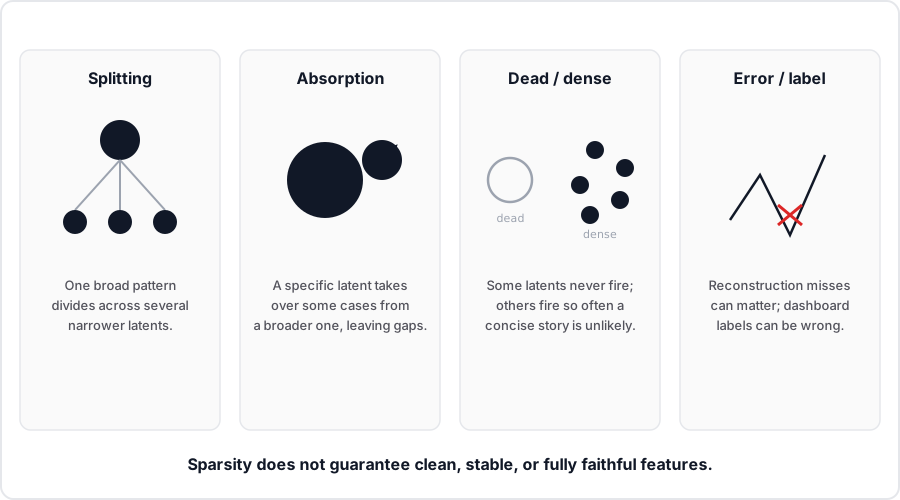
- Splitting divides one broad pattern across several narrower latents.
- Absorption gives a specific latent cases from a broader latent, leaving systematic gaps.
- Dead latents never activate on the evaluated distribution.
- Dense latents fire too broadly for a concise semantic description.
Notebook session
Open 1.3.3 Interpretability with SAEs. You can also use the solutions notebook.
Work through these sections in order:
- In 1️⃣ Intro to SAE Interpretability, complete:
- Intro to SAELens
- Visualizing SAEs with dashboards
- Running SAEs
- Replicating SAE dashboards, ending after Exercise: get top / bottom logits
- In Attention SAEs, run the setup cells through Exercise: explore attention SAE dashboards. That cell loads the
gpt2-small-hook-z-kkSAEs intoattn_saes, which the later exercises use. Exercise: derive attention DFA is optional. - Continue with Finding latents for features, then Ablation. Finish Exercise: find duplicate token features with ablation.
- Stop before Attribution patching.
- Return to the scaffold above and run the layer-9 experiment with latent 21474.
Optional notebooks
Write-up
Describe latent 21474 with examples from Neuronpedia. Include a minimal pair and a counterexample that tested your description. State the metric you chose before running the model. Report the ablation relative to the full SAE reconstruction, keeping your conclusion within the prompts and intervention you tested.
Be ready to contrast this evidence with what a probe or steering experiment would establish.
this week's practice
core
- Complete the core 1.3.3 sections through SAE dashboards and ablation
- Form and challenge a hypothesis for GPT-2 Small layer-9 latent 21474
- Choose a prompt-specific metric and controls
- Compare original, full reconstruction, and latent ablation, then write a bounded conclusion
stretch
- Optional deeper practice with 1.3.1 probes or 1.3.2 function vectors in Colab
- Optional Gemma/GemmaScope presenter demo
- Optional SAE failure-mode investigation or training