week 05 / 12
Finding circuits in language models
Use activation patching to test where GPT-2 Small carries information for the IOI task.
companion notebook · ARENA 1.4.1 and 1.4.2
new terms this week · 9
Causal methods
- Ablation
- Removing or replacing a model component to test whether a behavior depends on it.
- Activation patching
- Swapping activations between model runs to test which internals causally affect behavior.
- Noising vs. denoising
- Complementary patching experiments: noising corrupts a clean run to test necessity, while denoising restores part of a corrupted run to test sufficiency.
- Path patching
- A refinement of activation patching that isolates a specific sender-to-receiver path while holding the rest of the activation fixed.
Circuit analysis
- IOI
- Indirect Object Identification, a benchmark sentence task used to study a GPT-2 circuit.
- Name-mover head
- An attention head in the IOI circuit that attends to the correct name and copies it into the output logits.
- S-inhibition head
- An attention head in the IOI circuit that moves the "this name is duplicated" signal to the final position, reducing later heads' attention to the repeated subject name.
Metrics & attribution
- Logit difference
- A metric comparing model scores for the correct and incorrect answer tokens.
- Direct logit attribution
- Measuring how much each component’s direct residual-stream write changes the logit for a chosen token. It shows association, not cause.
This page takes you through the IOI circuit. It also covers the tools a researcher uses, from exploratory checks like attention patterns to more rigorous interventions like activation patching and path patching.
Week 5 assignment
Test one IOI activation patch
The required work uses GPT-2 small and fits on a Colab T4.
- Complete model & task setup in ARENA 1.4.1 and define the paired IOI prompts and logit-difference metric.
- Run or skim the supplied Section 2 helper cells needed by the next section. You do not need to complete the Logit Attribution exercises.
- Complete activation patching with modest batch sizes. Save one layer-by-position heatmap and one attention-head result.
- Record the clean, corrupted, and patched metric values. Explain what changed and give one reason the result might fail to generalize.
Keep the prompt set, model checkpoint, hook point, metric, baseline, and intervention fixed while comparing results. Reduce the prompt batch before changing the experiment if the T4 runs out of memory.
Slides: Finding circuits in language models
Indirect object identification
Early work in mechanistic interpretability either focused on simple behaviors in small models, or described complicated behaviors in larger models with broad strokes. In 2022, Wang et al. bridged this gap by explaining how GPT-2 small performs indirect object identification (IOI).1
An IOI prompt looks like this:
“When John and Mary went to the store, John gave a drink to” → “Mary”
Of the two names in the sentence, the model should predict the name that isn’t the subject of the last clause. GPT-2 small does this reliably. For patching, the corrupted twin flips only that repeated subject:
“When John and Mary went to the store, Mary gave a drink to”
The opening names stay put. Mary is now repeated, so the model prefers John. Both runs are still scored as logit(“ Mary”) − logit(“ John”), so the clean score is positive and the corrupted score flips sign.
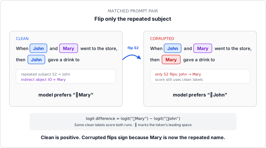
We can run that clean/corrupted contrast across several templates and many name pairs. One sentence can latch onto its wording, token positions, or those particular names. The original IOI study also keeps both names as single tokens, so the Mary-versus-John logit comparison stays unambiguous.
Logit difference
That Mary-versus-John score is the logit difference: the model’s logit for the clean prompt’s correct name minus its logit for the other name.
A positive value means the model favors the clean prompt’s answer. The corrupted run uses those same answer-token IDs, so when the model now prefers John, the score goes negative. The metric only compares those two names: another vocabulary token can still have the highest logit, and the score will not say so. Patching later uses the gap between the clean and corrupted values.
The function logits_to_ave_logit_diff below does that subtraction for a batch. Run the cell to score the eight-prompt set. Each row uses that prompt’s own correct name, so adjacent name-swapped sentences can both be positive.
Edit and run on this page. The first run loads GPT-2 and can take a minute. The table appears under the cell.
import json
import torch as t
from transformer_lens import HookedTransformer

model = HookedTransformer.from_pretrained(
    "gpt2-small", device="cpu", default_padding_side="left"
)
model.eval()
t.set_grad_enabled(False)

prompt_format = [
    "When John and Mary went to the shops,{} gave the bag to",
    "When Tom and James went to the park,{} gave the ball to",
    "When Dan and Sid went to the shops,{} gave an apple to",
    "After Martin and Amy went to the park,{} gave a drink to",
]
name_pairs = [
    (" Mary", " John"),
    (" Tom", " James"),
    (" Dan", " Sid"),
    (" Martin", " Amy"),
]
# Four templates × two name orders. Adjacent prompts swap the repeated subject.
prompts = [
    prompt.format(name)
    for prompt, names in zip(prompt_format, name_pairs)
    for name in names[::-1]
]
# answers[i] = (correct name, incorrect name) for prompts[i]
answers = [names[::i] for names in name_pairs for i in (1, -1)]
# answer_tokens: [batch, 2] integer IDs, column 0 correct, column 1 incorrect
answer_tokens = t.concat(
    [model.to_tokens(names, prepend_bos=False).T for names in answers]
)

# logits: [batch, seq, d_vocab] — one vocab score at every position
logits = model(model.to_tokens(prompts))

def logits_to_ave_logit_diff(logits, answer_tokens, per_prompt=False):
    """Correct-name logit minus incorrect-name logit, at the END position.

    logits:         [batch, seq, d_vocab]
    answer_tokens:  [batch, 2]  (correct id, incorrect id) per prompt
    per_prompt:     if True, return [batch]; if False, return the mean
    """
    # TransformerLens 2.11 pads on the right by default. The model above sets
    # default_padding_side="left", so index -1 is the last real token (END, ` to`)
    # for every prompt, even when prompts have different lengths.
    # That row is the next-token prediction. Shape: [batch, d_vocab]
    final_logits = logits[:, -1, :]
    # gather: look up a different pair of vocab IDs on each row.
    # answer_tokens[0] might be [5335, 1757] (" Mary", " John"); row 1 is the swap.
    # final_logits[:, 5335] would grab Mary for every prompt, which is wrong.
    # gather(dim=-1, index=answer_tokens) does: for batch item b, take
    #   [final_logits[b, answer_tokens[b, 0]], final_logits[b, answer_tokens[b, 1]]]
    # Shape: [batch, 2]
    answer_logits = final_logits.gather(dim=-1, index=answer_tokens)
    # unbind(dim=-1) splits that last axis: two tensors of shape [batch]
    # instead of one tensor of shape [batch, 2]. Then we can subtract them.
    correct_logits, incorrect_logits = answer_logits.unbind(dim=-1)
    answer_logit_diff = correct_logits - incorrect_logits
    return answer_logit_diff if per_prompt else answer_logit_diff.mean()

per_prompt_diff = logits_to_ave_logit_diff(logits, answer_tokens, per_prompt=True)
average_diff = logits_to_ave_logit_diff(logits, answer_tokens)

print("Per prompt logit difference:", per_prompt_diff)
print("Average logit difference:", average_diff)

payload = {
    "kind": "table",
    "title": "Logit differences",
    "columns": [
        {"label": "Prompt"},
        {"label": "Correct", "role": "correct"},
        {"label": "Incorrect", "role": "incorrect"},
        {"label": "Logit difference", "role": "metric"},
    ],
    "rows": [
        [prompt, repr(correct), repr(incorrect), f"{diff:.3f}"]
        for prompt, (correct, incorrect), diff in zip(prompts, answers, per_prompt_diff.tolist())
    ],
    "footer": {"label": "Average", "value": f"{average_diff.item():.3f}"},
}
print("__ARENA_TABLE__:" + json.dumps(payload, separators=(",", ":")))
Direct logit attribution
The logit difference is the one number that identifies how strongly the model prefers the correct name over the incorrect name. To see which residual writes produced that preference, direct logit attribution splits the same score across residual writes at END (the last token, to, where the model predicts the next name). That is how much each layer’s output already points toward the correct name. The residual stream is a running sum, so we can read that score after every layer. Run the cell to see it. Each point divides the accumulated stream by the full run's cached final LayerNorm scale, then projects it onto the logit-difference direction. The plot holds that normalization fixed. It does not rerun a model with the later layers removed, which would change the scale.
Edit and run on this page. The first run loads GPT-2 and can take a minute. The chart appears under the cell.
import json
import einops
import torch as t
from transformer_lens import HookedTransformer

model = HookedTransformer.from_pretrained(
    "gpt2-small", device="cpu", default_padding_side="left"
)
model.eval()
t.set_grad_enabled(False)

prompt_format = [
    "When John and Mary went to the shops,{} gave the bag to",
    "When Tom and James went to the park,{} gave the ball to",
    "When Dan and Sid went to the shops,{} gave an apple to",
    "After Martin and Amy went to the park,{} gave a drink to",
]
name_pairs = [
    (" Mary", " John"),
    (" Tom", " James"),
    (" Dan", " Sid"),
    (" Martin", " Amy"),
]
prompts = [
    prompt.format(name)
    for prompt, names in zip(prompt_format, name_pairs)
    for name in names[::-1]
]
answers = [names[::i] for names in name_pairs for i in (1, -1)]
answer_tokens = t.concat(
    [model.to_tokens(names, prepend_bos=False).T for names in answers]
)
tokens = model.to_tokens(prompts)
_, cache = model.run_with_cache(tokens)

# Unembed columns for the two names, then the direction that raises m.
answer_residual_directions = model.tokens_to_residual_directions(answer_tokens)
correct_dir, incorrect_dir = answer_residual_directions.unbind(dim=1)
logit_diff_directions = correct_dir - incorrect_dir  # [batch, d_model]

def residual_stack_to_logit_diff(residual_stack, cache, logit_diff_directions=logit_diff_directions):
    """Project residual vectors at END onto the logit-difference direction.

    residual_stack: [..., batch, d_model]  writes (or accumulated stream) at the last token
    Divide by the full run's cached final LayerNorm scale (held fixed for every
    layer), then average the dot product over the batch.
    """
    batch_size = residual_stack.size(-2)
    scaled = cache.apply_ln_to_stack(residual_stack, layer=-1, pos_slice=-1)
    return einops.einsum(
        scaled, logit_diff_directions, "... batch d_model, batch d_model -> ..."
    ) / batch_size

# Running sum of residual writes at END, after each attention (`_mid`) and MLP (`_pre`).
accumulated_residual, labels = cache.accumulated_resid(
    layer=-1, incl_mid=True, pos_slice=-1, return_labels=True
)
logit_lens_logit_diffs = residual_stack_to_logit_diff(accumulated_residual, cache)

print("labels:", labels)
print("logit diffs:", [round(value, 3) for value in logit_lens_logit_diffs.tolist()])

payload = {
    "kind": "chart",
    "title": "Logit difference from accumulated residual stream",
    "xLabel": "Layer",
    "yLabel": "Logit diff",
    "points": [
        {"label": label, "y": value}
        for label, value in zip(labels, logit_lens_logit_diffs.tolist())
    ],
}
print("__ARENA_CHART__:" + json.dumps(payload, separators=(",", ":")))
The score stays near zero until layer 7. Almost all of it arrives at attention layer 9, then layers 10 and 11 pull it back down. Attribution only sees a direct write onto the answer direction. A head in layer 7 or 8 can still carry the duplicated-name signal to END and look weak here. Activation patching tests those sites: replace the activation and measure whether the metric moves.
Activation patching
Activation patching copies one internal value from the clean run into the corrupted run. The rest of the forward pass continues, and we score the same logit difference. The experiment uses three forward passes:
- Run the clean prompt, cache the chosen activations, and record its logit difference.
- Run the corrupted prompt and record the corrupted baseline.
- Run the corrupted prompt again. At one layer, position, or head, replace the live activation with its clean cached value. Let the rest of the model continue and measure the patched output.
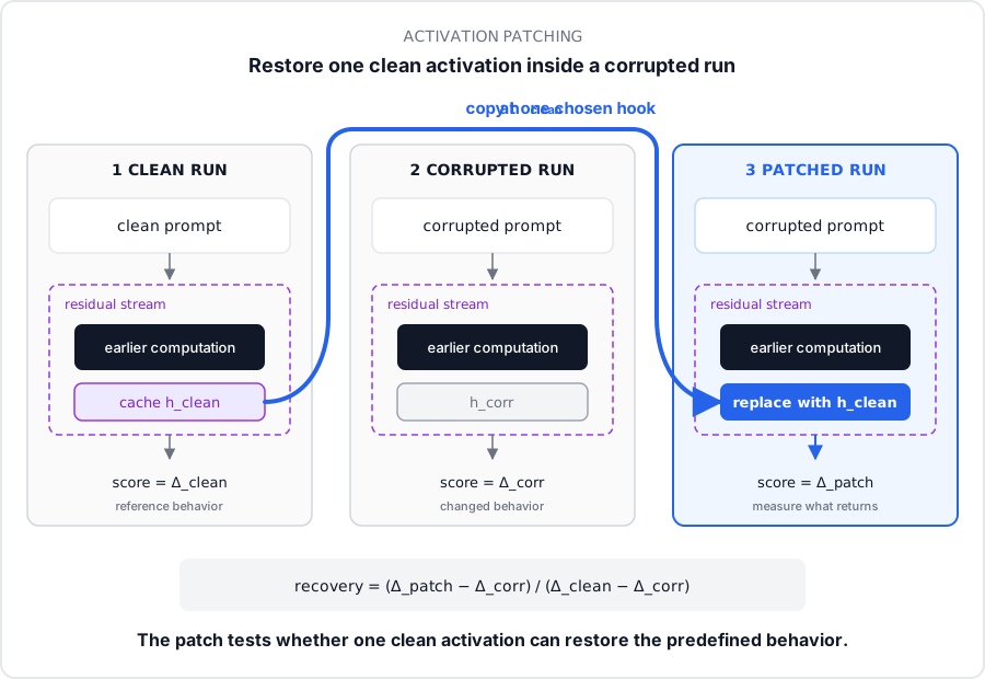
The patched score is:
Zero means the patch leaves the metric at the corrupted baseline. One means it restores the clean score. Values can fall below zero or exceed one because components interact and a patch can hurt or overcorrect. A small denominator makes the ratio unstable i.e. tiny changes in the patched metric then produce large swings in recovery.
The usual experiment is denoising: patch a clean activation into the corrupted run and see whether the clean answer returns. The reverse experiment, called noising, puts a corrupted activation into the clean run. A successful denoising patch shows that the clean value can restore task-relevant information through this corruption; a successful noising patch shows that replacing the value can disrupt the clean computation. Redundant components may compensate, so these experiments are not formal proofs of sufficiency or necessity.
A single patch tests one chosen site. Direct logit attribution already pointed at late writes at END, but it can miss earlier routing, so a sweep searches more broadly: every layer and position, then every attention head. The heatmap localizes where the clean and corrupted runs differ in ways that affect the metric.
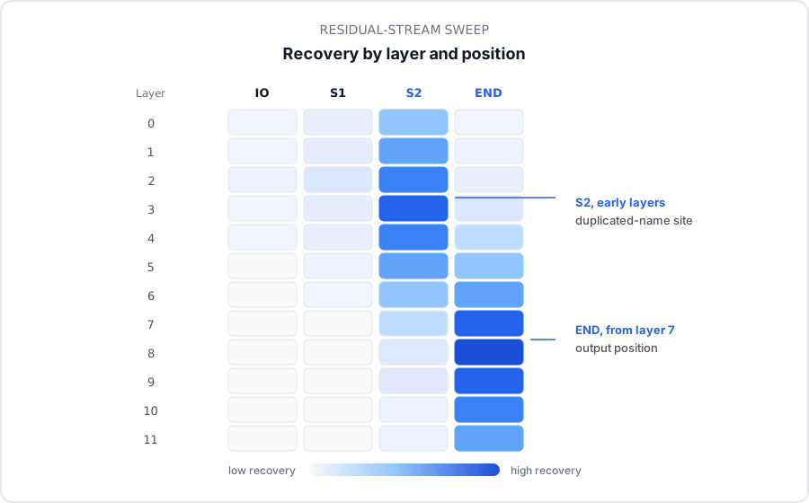
A bright cell gives you a place to investigate. The same information can persist across neighboring residual-stream sites, so a cluster of bright cells need not represent several distinct computations. Patching may also create an unusual combination of activations. Before naming a mechanism, repeat the result across prompt templates and zoom in with head-level tests or the reverse patch direction.
The two bright regions already sketch a circuit. Early layers mark the duplicated name at S2. Later layers write the remaining name at END.
The IOI circuit
The IOI paper used multiple methods (attribution, activation patching, path patching, and ablation) to identify a 26-head circuit in GPT-2 small. Its central path follows a compact algorithm:
- Identify previous names, then mark the duplicated subject.
- S-inhibition heads remove that duplicated name from later attention.
- Name-mover heads attend to the remaining name and write it toward the output.
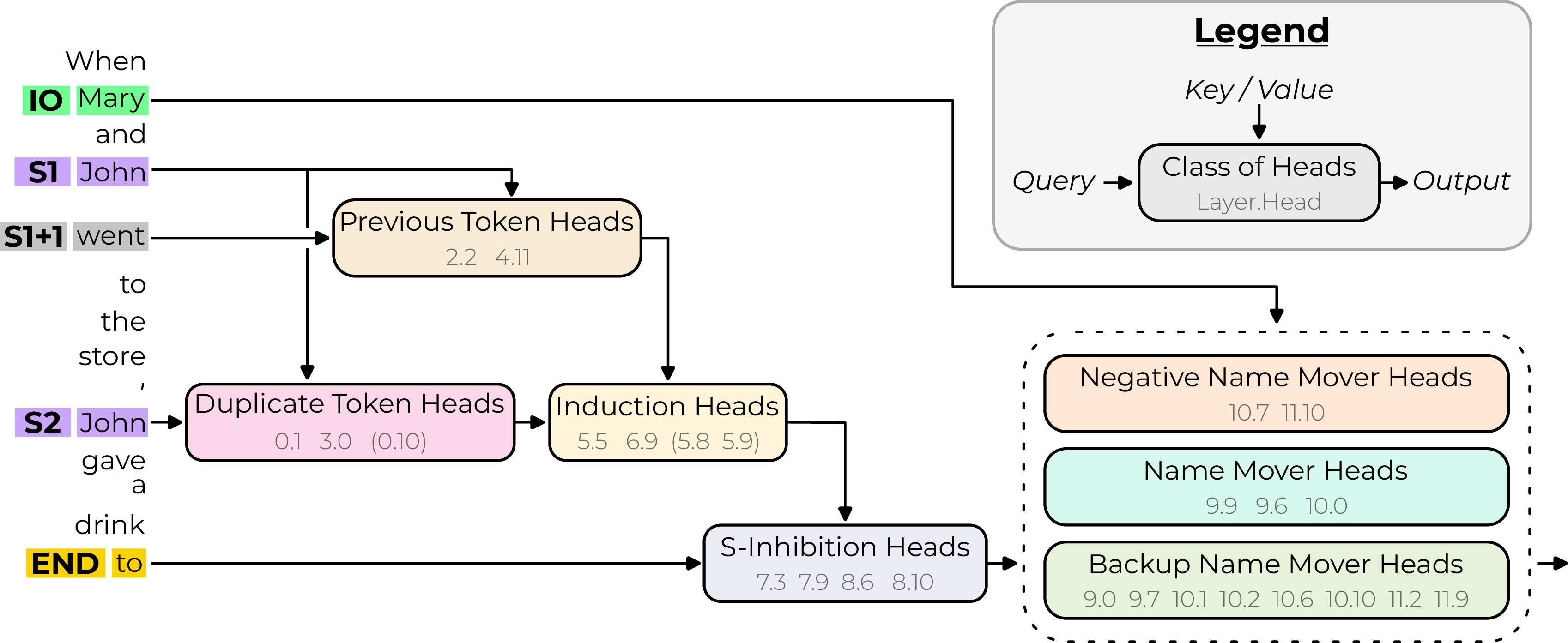
The full circuit includes negative name-mover heads that push against the correct answer. It also has backup name movers that compensate when researchers ablate the primary heads. This compensation can be easy to miss as the model can respond to an intervention by changing its downstream computation, which makes a single ablation understate the component's normal role.
Path patching narrows the intervention from a whole node to one proposed sender-to-receiver route while controlling competing routes. For example, you can test whether an S-inhibition head changes the score through a particular name mover. This isolates the route more precisely than a node patch. The result still belongs to the prompts, metric, and control values used in the experiment.
SAE circuits
Attention heads give the IOI analysis a manageable set of components. A larger model contains many more heads and MLP computations. Last week, sparse autoencoders decomposed one activation into SAE latents. Those latents can serve as candidate circuit nodes.
For one prompt, a latent-to-latent gradient measures how a small change in an earlier latent would change a later latent. Token-to-latent and latent-to-logit gradients connect those internal nodes to the input and output. Multiplying a local gradient by the source activation gives an attribution score for one possible edge.
This score comes from a local linear approximation around one forward pass. Large interventions may behave differently, especially when features interact. Treat a high-scoring edge as an experiment to run next, then ablate or swap the source latent and measure what happens.
Transcoders and attribution graphs
A standard SAE reconstructs activations at one hook point. A transcoder instead learns a sparse mapping from a layer’s input to that layer’s output. Each active transcoder latent has a direction that reads from the residual stream and a direction that writes back, so its connections to earlier and later nodes are easier to trace.
An attribution graph connects input tokens, active SAE or transcoder latents, model errors, and output logits for one prompt. The graph keeps high-influence nodes and edges after locally approximating the model’s computation. It gives a testable account of how information could flow from this input to this output.
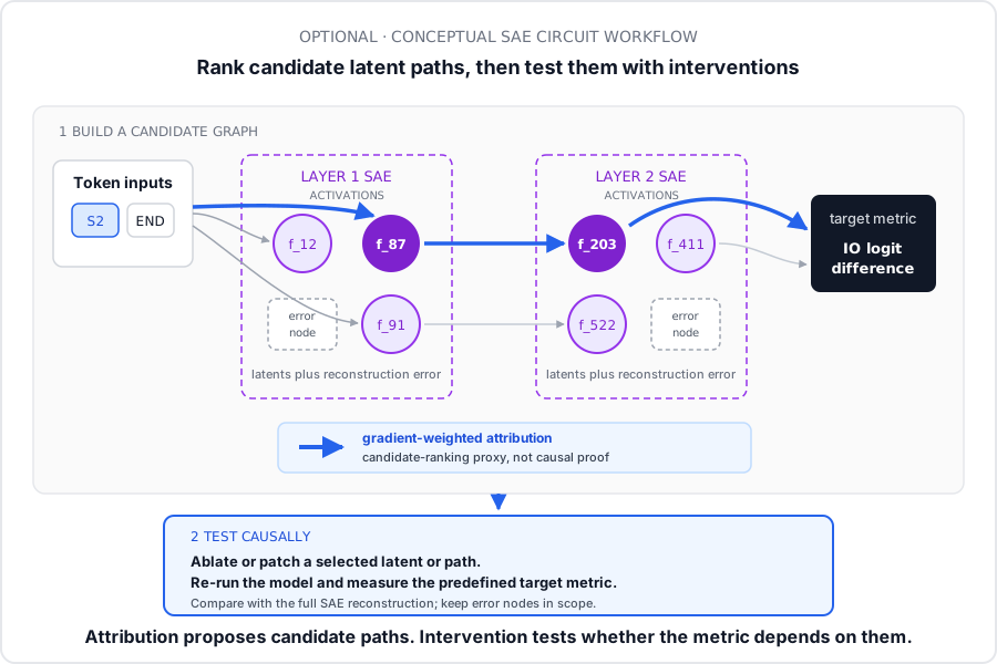
An attribution graph is a compressed view of the model, and the missing pieces matter. SAE latents can split one feature or combine several; reconstruction error leaves computation outside the sparse nodes. Local approximations may also fail after a large edit, while pruning can discard weak edges that matter together. Check the error terms, compare with the unmodified model, and test the proposed graph by ablating or swapping features.
The attribution graphs in Circuit Tracing (Anthropic, 2025) come from a local replacement model that freezes the original run's attention patterns and normalization denominators. Their edges show how values flow under that fixed routing. They do not explain how the model chose where each attention head attends.
Circuit evidence
The methods fit together because each one sets up a different next step:
| What you learn | Useful next check | |
|---|---|---|
| Attention pattern | Where a head reads on these prompts | Patch or ablate the head and measure the output |
| Direct logit attribution | Which direct residual writes align with the answer | Look for indirect effects through later components |
| Activation patching | Whether replacing one node changes the metric | Narrow the sweep to heads, positions, or paths |
| Path patching | Whether a chosen sender-to-receiver route matters under the controls | Change the controls and test the route on new prompts |
| Attribution graph | A sparse, input-specific computation worth testing | Measure reconstruction error and intervene on its features |
| Feature intervention | How a latent edit changes behavior in this setup | Check whether the edit stays in distribution and whether the latent has a stable meaning |
Start with the behavior and metric, use observational tools to find a promising site, and then intervene. If a component survives those tests, try removing everything outside the proposed circuit. Failures and compensatory effects are useful results too; they often reveal the part of the computation your first diagram missed.
review quiz
Notebook session
Open the current 1.4.1 Indirect Object Identification exercises. The solutions notebook can help when an implementation detail blocks the patching experiment.
Required work:
- Select a T4 GPU if Colab offers one. An A100 is not required.
- Complete 1️⃣ Model & Task Setup.
- Skim 2️⃣ Logit Attribution and run its supplied helper code. Skip its exercises.
- In 3️⃣ Activation Patching, run the setup under Creating a metric. It defines
clean_tokens,corrupted_tokens,clean_cache, andcorrupted_cache, plus the baselinesclean_logit_diffandcorrupted_logit_diff. - Complete the rest of 3️⃣ Activation Patching. Use modest prompt batches and save the layer-by-position and attention-head results.
- Stop before 4️⃣ Path Patching.
Optional work:
- Complete the Logit Attribution exercises, then compare their observational scores with patching effects.
- Continue through Path Patching, Full Replication, or the anomaly investigations in 1.4.1.
- Open 1.4.2 SAE Circuits exercises or its solutions. Most non-Gemma exercises can run on free Colab, but the notebook is much heavier than the core assignment. The Gemma portions may need more memory.
Write-up
Submit one short patching report with:
- The prompt distribution, model checkpoint, and logit-difference metric.
- One activation-patching heatmap and one attention-head result.
- The clean, corrupted, and patched metric values and the patch direction.
- Your conclusion, including the tested site, prompts, metric, and one reason the result might change in a broader experiment.
Sources
- ARENA 1.4.1: Indirect Object Identification
- ARENA 1.4.2: SAE Circuits
- Interpretability in the Wild: a Circuit for Indirect Object Identification in GPT-2 Small
- Transcoders Find Interpretable LLM Feature Circuits
- Circuit Tracing: Revealing Computational Graphs in Language Models
Footnotes
this week's practice
core
- Complete 1.4.1 Model & Task Setup
- Run or skim the supplied Section 2 helper cells
- Complete Activation Patching on GPT-2 Small using a Colab T4 if available
- Report one heatmap, one attention-head result, and a bounded conclusion
stretch
- Complete the Logit Attribution exercises
- Continue through Path Patching, Full Replication, or anomaly investigations
- Explore 1.4.2 SAE Circuits, transcoders, and attribution graphs