week 07 / 12
Reinforcement learning foundations
How agents learn from consequences. Sometimes with a map. Sometimes by stumbling forward.
companion notebook · ARENA 2.1 Sections 1–2
new terms this week · 19
Reinforcement learning
- State
- The information needed from the past to determine the distribution of the next state and reward once an action is given.
- Markov decision process
- A model of sequential decisions built from states, actions, transition probabilities, rewards, and a discount factor.
- Policy
- A rule or probability distribution that chooses an action from a state.
- Trajectory
- One sequence of states, actions, and rewards produced as an agent interacts with an environment.
- Episode
- A finite sequence of interactions between an agent and an environment.
- Discounted return
- The sum of future rewards after multiplying later rewards by progressively smaller powers of the discount factor.
- Discount factor
- A number between zero and one that controls how strongly an agent values later rewards.
- Value function
- The expected discounted return from a state under a policy.
- Q-value
- The expected discounted return after taking a chosen action in a state and following a policy afterward.
- Bellman equation
- A recursive equation that writes a value as immediate reward plus the discounted value of what follows.
- Tabular method
- A reinforcement learning method that stores one value for every state or state-action pair.
- Q-learning
- An off-policy method that updates a Q-value toward the reward plus the best estimated value at the next state.
- SARSA
- An on-policy method that updates a Q-value using the next action selected by the current policy.
- TD error
- The difference between a current value estimate and its one-step reward-plus-next-value target.
- Epsilon-greedy
- A policy that usually takes the highest-value action and chooses a random action with probability epsilon.
- DQN
- Deep Q-Network: a neural network trained to estimate Q-values for each action.
- Replay buffer
- A store of past transitions sampled to train a reinforcement learning agent.
- Policy gradient
- A method that changes policy parameters in the direction that raises expected return.
Tools
- Gymnasium
- A Python library that provides standard reinforcement learning environments and interfaces.
Week 7 notebook
Week 7 notebook
- Open the exercise notebook. Use the solutions notebook to check your work.
- Complete Section 1 through the Norvig penalty experiment, which uses a small stochastic gridworld to show how step costs change the best policy.
- Complete Section 2 through CliffWalking, including .
- Stop before the Section 2 bonus exercises and Section 3.
- Run the notebook on CPU.
Slides: Reinforcement learning foundations
How do you teach a lander to touch down? You can write rules for when each engine should fire, as in the left example below. The controller on the right learned through practice. In one training run of about 1.5 million simulated steps (no log is linked), a neural network chose how to fire the engines. After each batch of attempts, training adjusted the network so actions that earned more reward became more likely.
Hand-written rules

Learned from reward

As tasks grow, writing a rule for every situation stops scaling. Large language models can produce countless possible responses. The agent-environment loop captures how learning from feedback works one step at a time.
The agent-environment loop
In reinforcement learning (RL), an agent chooses actions in an environment and learns from the rewards that follow. At step , it receives an observation, chooses action , then receives reward and the next observation. The loop supplies consequences rather than labels, so learning must relate each consequence to the action and situation that produced it.
The environment's state contains enough information from the past to determine the probabilities of the next state and reward once an action is fixed. An observation is the information about that state available to the agent, so it may reveal the full state or only part of it. This lesson's environments reveal the full state, which lets us write each observation as . Their fixed sets of discrete actions also fit in tables.
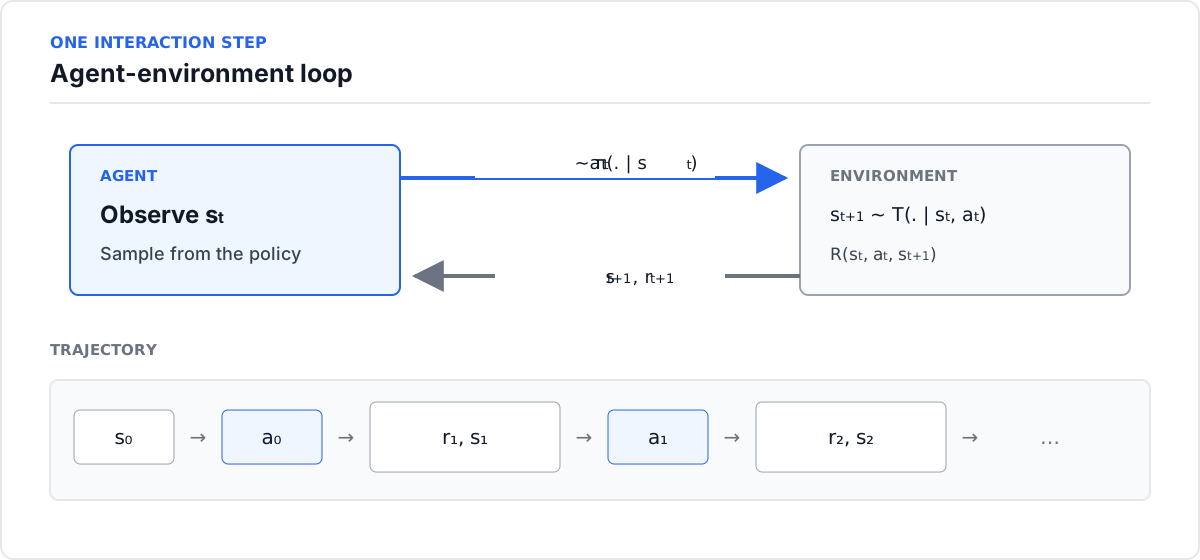
From each state, a policy chooses an action deterministically or assigns each action a probability. We write the probability of action in state as . Following a policy produces a trajectory of states, actions, and rewards:
A return combines a trajectory's rewards into one score. The agent maximizes that score in expectation across possible outcomes. The discounted return weights rewards from step onward: add the next reward, then times the following reward, then times the reward after that:
The discount factor controls how much later rewards count. Low values favor near rewards, while high values retain more weight on later rewards. Bounded rewards give a finite discounted return when the discount factor is at least 0 but less than 1 (). At , a continuing sequence such as 1, 1, … has an infinite sum, so this objective cannot distinguish such sequences without a finite horizon or another criterion.
To compare starting states under policy , the value function gives the expected discounted return from state under that policy:
The expectation averages over the policy's actions and the environment's outcomes, conditioned on starting in . This gives one value for the state under . Improving the policy requires comparing the available actions, so the action value fixes the first action as , then follows .
Markov decision processes
Calculating state and action values from the environment's rules requires its transition probabilities and rewards. A finite Markov decision process (MDP) specifies these rules along with the states and actions. The Toy MDP puts states L, C, and R in a line. The agent starts at C, chooses left or right, and must account for rewards that arrive after leaving the middle. Its rules specify:
- Transition probabilities for reaching each next state from state after action .
- Rewards for each move.
- The discount factor .
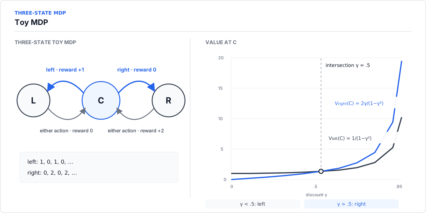
From C, left moves to L and pays +1; right moves to R and pays 0. From L, either action returns to C and pays 0. From R, either action returns to C and pays +2. Every transition continues the loop because the Toy has no terminal state.
The choice at C shows how discounting changes decisions. Always choosing left from C produces rewards of 1, 0, 1, 0, …. Always choosing right produces 0, 2, 0, 2, …. Discounting weights each reward by a power of γ, so the returns expand term by term:
Each series repeats every two steps. The zero-valued terms add nothing, and each remaining term equals the previous one times . This repeated-power pattern is a geometric series. The formula rewrites its infinite sum as a fraction. Here :
The better policy depends on γ. With a low γ, the always-left policy's immediate reward of 1 outweighs the later reward of 2. With a high γ, the always-right policy preserves enough of that later reward to make waiting worthwhile. The policies tie at .
Animation: sweep γ across the Toy MDP values

The 200-step rollouts approximate the infinite-horizon values. Always-left wins below , always-right wins above it, and the policies tie at the crossover.
The formulas describe whole reward sequences, while the model arrays encode one transition at a time. Both arrays have shape (num_states, num_actions, num_states), with axes for current state, action, and next state. The code's s_next matches . T[s, a, s_next] stores the transition probability , and R[s, a, s_next] stores the corresponding reward. The next-state probabilities in T[s, a, :] sum to one.
NumPy is preinstalled.
import json
import numpy as np

T = np.zeros((3, 2, 3))
R = np.zeros((3, 2, 3))
# states: L=0, C=1, R=2; actions: left=0, right=1
transitions = [
    (0, 0, 1, 0), (0, 1, 1, 0),
    (1, 0, 0, 1), (1, 1, 2, 0),
    (2, 0, 1, 2), (2, 1, 1, 2),
]
for s, a, s_next, reward in transitions:
    T[s, a, s_next] = 1
    R[s, a, s_next] = reward

print(T.shape, R.shape)
print(T.sum(axis=-1))
assert np.allclose(T.sum(axis=-1), 1)
row_labels = [f"{state} · {action}" for state in ["L", "C", "R"] for action in ["left", "right"]]
payload = {
    "kind": "arrays",
    "arrays": [
        {
            "name": "T · transition probability",
            "axisLabel": "rows: current state/action · columns: next state L/C/R · shape (3, 2, 3)",
            "palette": "blue",
            "rowLabels": row_labels,
            "columnLabels": ["L", "C", "R"],
            "values": T.reshape(-1, T.shape[-1]).tolist(),
        },
        {
            "name": "R · reward",
            "axisLabel": "rows: current state/action · columns: next state L/C/R · shape (3, 2, 3)",
            "palette": "amber",
            "rowLabels": row_labels,
            "columnLabels": ["L", "C", "R"],
            "values": R.reshape(-1, R.shape[-1]).tolist(),
        },
    ],
}
print("__ARENA_ARRAYS__:" + json.dumps(payload, separators=(",", ":")))
# (3, 2, 3) (3, 2, 3)
# [[1. 1.]
#  [1. 1.]
#  [1. 1.]]
For the deterministic Toy, T[s, a, :] assigns probability 1 to the single resulting next state and 0 to every other state. If state s and action a can produce several outcomes, the transition is stochastic: the row assigns each possible next state a probability, and those probabilities sum to 1.
Tabular planning with policy iteration
With T and R encoded, the Bellman equation computes each infinite-horizon value one transition at a time. To value a state, add the reward you expect from the next step to the discounted value of wherever the agent lands:
In symbols, weights each action, and weights each possible next state. supplies the reward for the move, and discounts the value of that next state:
Known and let us calculate from . The calculation averages the reward and discounted value of each possible next state:
Policy evaluation computes the values of a fixed policy. The iterative method starts from guessed values, updates every state from the previous values, and stops when the largest change falls below a chosen tolerance. Exact evaluation solves the same equations directly. The evaluate function compares the numerical and exact results, which should agree.
The two methods should differ by less than one millionth.
import numpy as np

T = np.zeros((3, 2, 3)); R = np.zeros_like(T)
for s, a, sn, r in [(0,0,1,0),(0,1,1,0),(1,0,0,1),
                    (1,1,2,0),(2,0,1,2),(2,1,1,2)]:
    T[s, a, sn], R[s, a, sn] = 1, r

def evaluate(policy, gamma=0.99, tol=1e-12):
    P = T[np.arange(3), policy]
    rewards = (P * R[np.arange(3), policy]).sum(axis=1)
    exact = np.linalg.solve(np.eye(3) - gamma * P, rewards)
    numerical = np.zeros(3)
    while True:
        updated = rewards + gamma * P @ numerical
        if np.max(np.abs(updated - numerical)) < tol:
            break
        numerical = updated
    return updated, exact

answers = []
for policy in (np.array([0, 0, 0]), np.array([0, 1, 0])):
    numerical, exact = evaluate(policy)
    answers.append(float(numerical[1]))
    assert np.max(np.abs(numerical - exact)) < 1e-6
print([round(x, 4) for x in answers])
# [50.2513, 99.4975]
Policy improvement computes each action's Q-value and chooses a highest-value action in every state, a step called greedy improvement. The resulting greedy policy improves or preserves the value at every state. Policy iteration alternates evaluation and improvement until the policy stops changing. This stable greedy policy is optimal. Ties can produce several optimal policies with the same value, so the implementation's tie-breaking rule (select the first action among those with the highest value) can change the returned arrows.
We apply policy iteration to the Norvig environment, a small 3 by 4 stochastic gridworld with a goal, a trap, and a wall. Movement can slip away from the selected direction, so the best policy balances route length, step costs, and the risk of entering the trap.
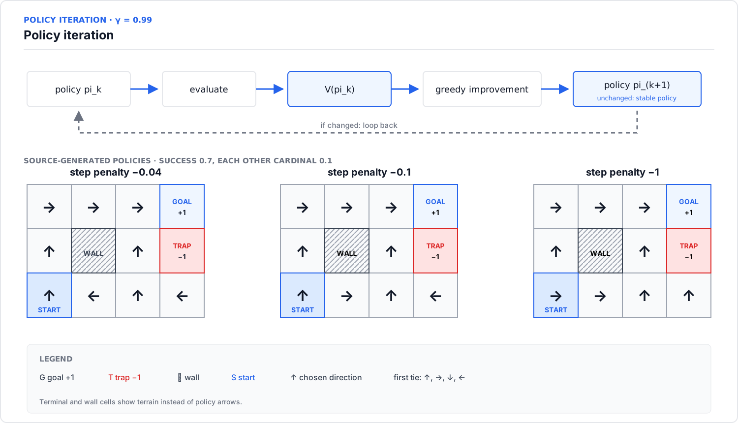
-1 the policy passes beside the trap to end sooner. Equal-value actions follow the source's first-argmax order: up, right, down, left.The map uses S for the start, G for the goal, T for the trap, and # for the wall:
Reaching G ends the episode with +1, while reaching T ends it with -1. The wall blocks movement. The default reward for a step that continues the episode is -0.04. The agent can move up, right, down, or left. Its intended direction occurs with probability 0.7, and each of the other three directions occurs with probability 0.1. A move into the wall or boundary leaves the state unchanged.
The penalty experiment tests how repeated step costs change the best route. Run policy iteration with -0.04, -0.1, and -1, then compare the generated routes. Small costs can support a longer route around the trap. At -1, ending quickly can cost less than taking extra steps. The transition model and tie-breaking rule determine the exact arrows.
Gymnasium and sampled experience
Known transition (T) and reward (R) tables let the Bellman equations average over every possible next state. When those tables are unavailable, a gymnasium environment supplies sampled outcomes through a standard API. reset() starts an episode and returns (observation, info). step(action) returns (observation, reward, terminated, truncated, info), containing the next observation, reward, two stopping flags, and extra information. An observation may expose the underlying state or only part of it.
terminated marks an ending defined by the MDP. truncated marks an external cutoff such as a time limit. The interaction loop stops when either is true and handles both flags outside the Experience record. That record stores the current observation (obs), action (act), reward, next observation (new_obs), and optional next action (new_act). An agent owns the environment and random generator, runs the loop, and delegates action selection and updates; the cell below makes both stopping flags concrete.
The FrozenLake gridworld below has a one-row map with S for the start, F for a safe frozen tile, and G for the goal. A short rollout demonstrates both flags: RIGHT reaches the goal, while LEFT is blocked at the starting boundary until TimeLimit truncates the episode.
Gymnasium 0.29.1 is preinstalled. This FrozenLake map is deterministic.
from dataclasses import dataclass
from typing import Optional

import gymnasium as gym

@dataclass
class Experience:
    obs: int
    act: int
    reward: float
    new_obs: int
    new_act: Optional[int] = None

env = gym.make("FrozenLake-v1", desc=["SFG"], is_slippery=False, max_episode_steps=3)

def run_episode(label, actions):
    obs, info = env.reset()
    print(label, "reset", (obs, info))
    for action in actions:
        new_obs, reward, terminated, truncated, info = env.step(action)
        print("step", (new_obs, reward, terminated, truncated, info))
        experience = Experience(obs, action, reward, new_obs)
        print(experience)
        if terminated or truncated:
            break
        obs = new_obs

run_episode("goal", [2, 2])  # RIGHT
run_episode("time limit", [0, 0, 0])  # LEFT, blocked
env.close()

# goal reset (0, {'prob': 1})
# step (1, 0.0, False, False, {'prob': 1.0})
# Experience(obs=0, act=2, reward=0.0, new_obs=1, new_act=None)
# step (2, 1.0, True, False, {'prob': 1.0})
# Experience(obs=1, act=2, reward=1.0, new_obs=2, new_act=None)
# time limit reset (0, {'prob': 1})
# step (0, 0.0, False, False, {'prob': 1.0})
# Experience(obs=0, act=0, reward=0.0, new_obs=0, new_act=None)
# step (0, 0.0, False, False, {'prob': 1.0})
# Experience(obs=0, act=0, reward=0.0, new_obs=0, new_act=None)
# step (0, 0.0, False, True, {'prob': 1.0})
# Experience(obs=0, act=0, reward=0.0, new_obs=0, new_act=None)
The Random and Cheater reference agents test the interaction loop before learning begins. Random samples actions without updating values. Cheater reads the environment model, computes an optimal policy, and follows it. On ToyGym-v0, Cheater should earn a higher average discounted return than Random. This comparison checks the interaction loop and reward accounting.
Tabular learning with Q-learning and SARSA
With the interaction loop checked, a learner estimates action values from sampled transitions when T and R are unavailable. It must try actions whose values remain uncertain because repeatedly choosing the current best action can hide a better one. An epsilon-greedy policy chooses a random action with probability epsilon. With the remaining probability, it chooses the action with the highest estimated value. If several actions tie, the implementation chooses the first one. Every action starts with value zero, so an agent with no exploration first picks action 0. Whether it keeps repeating that action depends on the reward. In the ExplorationGrid-v0 example below, ordinary moves earn 0, so the update leaves every value at zero, the tie persists, and the agent repeats the first action. A negative reward breaks the tie: an update that turns [0, 0, 0, 0] into [-0.1, 0, 0, 0] makes the next argmax pick action 1.
The target is the new estimate that the current Q-value moves toward. It combines the observed reward with a discounted estimate of later reward. Two learning algorithms, Q-learning and SARSA, use the same observed reward but estimate the continuation from different actions. The TD error is the target minus the current Q-value. The learning rate controls how far the Q-value moves toward that target. A terminal transition has no later value, so its estimate of the continuation is zero:
Q-learning uses the largest next-state value. Its target evaluates the greedy next action even when the policy collecting experience selects another action. This makes Q-learning off-policy. SARSA uses the next action selected by the policy collecting experience. This makes SARSA on-policy. Its name follows the sequence state, action, reward, state, action. The update preserves that sampled next action:
- Select
a_next. - Store it as
new_actin theExperiencerecord. - Compute the target.
- Update the current Q-value.
- Continue from the same action.
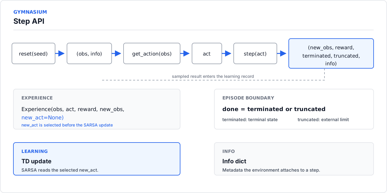
terminated marks an environment terminal state, while truncated marks an external limit. SARSA selects and stores new_act before constructing the target, then continues with that action.ExplorationGrid-v0 is a deterministic 5 by 5 gridworld. The agent starts at S, can move up, right, down, or left, and stops at the goal G for +1 or the trap T for -1. Other moves give 0. The simulator makes the Q-learning and SARSA bootstrap choices visible one update at a time.
Tabular update lab
Temporal-difference update
alpha = 0.10 gamma = 0.99 Step through the deterministic ExplorationGrid. Q-learning bootstraps from the best next action. SARSA bootstraps from the action its epsilon-greedy policy actually selects.
ExplorationGrid-v0
Deterministic 5 by 5 grid
Table lookup
Bootstrap target
Q(current state, ·)
Q(next state, ·)
Take one step to compare the two bootstrap rules.
One update
target = reward + gamma × bootstrap
waiting for a transition - old Q
- 0.000
- reward
- 0.000
- bootstrap
- 0.000
- target
- 0.000
- TD error
- 0.000
- new Q
- 0.000
new Q = old Q + 0.10 × TD error
The table starts at zero. With epsilon 0, first-maximum tie-breaking sends the agent up until it sticks at the top wall.
Reset the simulator, then switch algorithms while keeping the same seed and epsilon to compare the same sampled transition. Q-learning bootstraps from the maximum entry in Q(s_next). SARSA bootstraps from the entry for the sampled next action, which can change with epsilon even before any Q-value changes.
To see how exploration affects learning, Q-learning uses this map with four exploration rates (epsilon): 0, 0.1, 0.2, and 0.5. An exploration rate of 0 means the agent never chooses a random move. A rate of 0.5 means it does so half the time.
Each setting runs five times to reduce the effect of luck. In each run, the agent gets 100 episodes to learn, and every action starts with the same estimated value. Each episode stops after 100 moves. The comparison tracks the average discounted reward earned so far.
Without exploration, all actions initially look equally good. The tie-breaking rule chooses up, so the agent reaches the top wall and keeps trying to move through it. It never earns a reward. Moderate exploration (0.1 or 0.2) helps the agent find and repeat a route to the goal. At 0.5, random moves disrupt that route more often, so later rewards remain lower.
Eligibility traces
One-step TD updates only the latest state-action pair. When a reward arrives several moves later, earlier choices learn about it only as that information moves backward one transition at a time. An n-step target moves it farther by including the next n rewards before bootstrapping from a later value. The λ-return blends targets of different lengths, giving longer targets more weight as λ increases. At λ = 0, it reduces to one-step TD. At λ = 1, it becomes the full return for a terminating episode with zero future value.
The agent keeps a temporary weight for each recently visited state-action pair. These weights shrink after each step. When a new TD error arrives, they determine how much each earlier choice is updated. Eligibility traces store the weights in a table E, shaped like Q. With accumulating traces, each visit adds one to a pair's weight, and E resets to zero at the start of each episode. This backward flow is called the backward view of the λ-return.
For each transition, SARSA(λ) uses the usual SARSA TD error, with future Q set to zero at a terminal state:
- Calculate the TD error.
- Add one to the current pair's trace.
- Update every Q-value according to its trace.
- Multiply every weight by so it shrinks over time.
The discount factor and lambda together control how quickly the weights shrink. Repeated visits can make accumulating traces large, so slow decay combined with a large learning rate can destabilize the updates.
Both runs use the same transitions and differ only in λ.
import numpy as np

def two_updates(lam):
    Q = np.zeros((3, 2)); E = np.zeros_like(Q)
    for s, a, reward, sn, an in [(0, 0, 1, 1, 1), (1, 1, 2, 2, 0)]:
        delta = reward + 0.9 * Q[sn, an] - Q[s, a]
        E[s, a] += 1
        Q += 0.5 * delta * E
        E *= 0.9 * lam
    return Q

traced, one_step = two_updates(0.8), two_updates(0.0)
print(traced[[0, 1], [0, 1]])
print(one_step[[0, 1], [0, 1]])
assert np.allclose(traced[[0, 1], [0, 1]], [1.22, 1.0])
assert np.allclose(one_step[[0, 1], [0, 1]], [0.5, 1.0])
# [1.22 1.  ]
# [0.5 1. ]
After the first update, the earlier pair is worth 0.5 in both runs. With λ = 0.8, its remaining weight carries part of the second TD error back and raises the value to 1.22. With λ = 0, the weight has shrunk to zero, so the value stays at 0.5.
LargeGrid tests the same effect over a longer route. The agent crosses an empty 8 by 8 grid from the bottom-left to a goal at the top-right. The shortest route takes 14 moves, and only the goal pays +1.
Across five runs and 150 episodes, one-step SARSA and SARSA(λ) use the same settings. With λ = 0.8, the goal's TD error can update earlier choices from that route in the same episode, so the comparison tests whether returns improve sooner.
After testing faster reward propagation, CliffWalking returns to Q-learning and SARSA to test target choice when exploration is costly.
CliffWalking
CliffWalking places a 4 by 12 grid between the agent and a goal. The bottom row contains the start, a long cliff, and the goal. Stepping into the cliff gives a large penalty and returns the agent to the start. A path along the cliff edge is short and exposed to epsilon-greedy mistakes. A route one row higher takes extra steps and reduces that risk.

-13 along the cliff edge, while the displayed SARSA policy returns -17 on a longer route with more clearance.The comparison uses one 500-episode run with gamma = 1, epsilon = 0.1, alpha = 0.1, and every Q-value initialized to zero. Here gamma = 1 sums rewards without discounting. Q-learning's target uses the best predicted next action and favors the short route. SARSA's target uses the epsilon-greedy action sampled during training, so it accounts for exploratory cliff falls and learns a safer route.
SARSA has the higher return during epsilon-greedy training, where random exploratory actions can incur cliff penalties. Final greedy evaluation disables exploration and always chooses the action given by argmax Q, measuring the greedy policy encoded by the learned values. Its return depends on the seed and implementation. The figure illustrates this distinction with one run.
Further reading
- The ARENA 2.1 exercise notebook contains the tests, experiments, and starter code used here.
- The ARENA Introduction to RL lesson presents the notebook material in web-lesson form.
- OpenAI's Spinning Up introduction to reinforcement learning develops the agent-environment framework, return objective, value functions, and Bellman equations.
- Sutton and Barto, Reinforcement Learning: An Introduction, second edition, develops dynamic programming, temporal-difference control, eligibility traces, and CliffWalking in full.
this week's practice
core
- Complete 2.1 Section 1 Planning through the Norvig penalty experiment
- Complete 2.1 Section 2 Learning through CliffWalking, including SARSA(lambda)
- Pass the supplied tests and compare online exploratory reward with final greedy return