week 03 / 12
Introduction to mechanistic interpretability
Use TransformerLens to inspect activations, test attention patterns, and identify induction heads.
companion notebook · ARENA 1.2
new terms this week · 7
Interpretability foundations
- Mechanistic interpretability
- The project of explaining model behavior by identifying the internal algorithms and components that cause it.
Tools
- TransformerLens
- A library that exposes transformer activations and hooks for mechanistic interpretability work.
- Activation cache
- A collection of named intermediate activations recorded during a model forward pass.
- Hook
- A function called at a named activation during a forward pass to read or replace that activation.
Circuit analysis
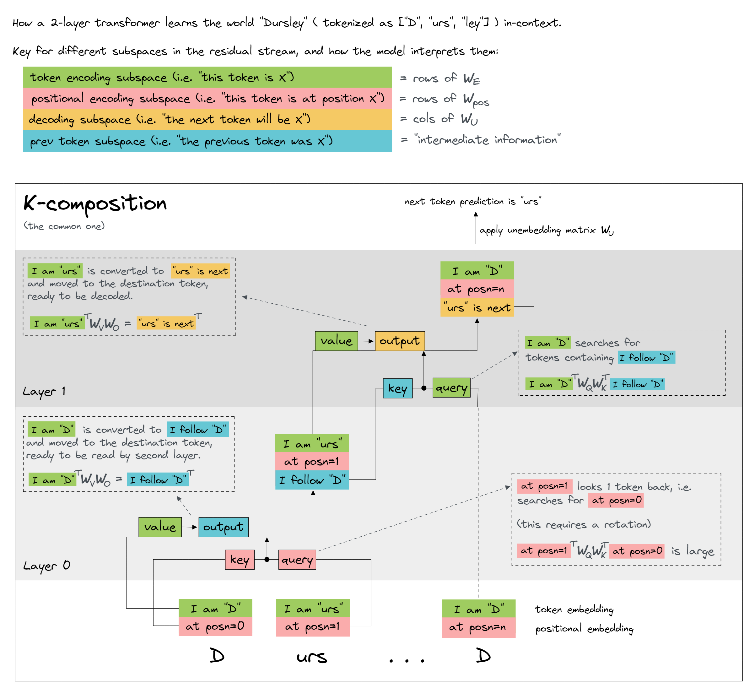
- K-composition
- A circuit in which one attention head builds its keys from information written by an earlier head.
- Induction head
- An attention head that implements a "copy what followed this token last time" pattern.
Metrics & attribution
- Induction score
- The average attention weight on the expected offset stripe for destinations in the second copy of a repeated sequence.
Week 2 followed tokens through attention and the residual stream to next-token logits. This lesson defines the induction problem, then uses TransformerLens to inspect it.
The modern circuits program began in vision models, where researchers like Olah et al. combined feature visualization, dataset examples, weight analysis, and interventions to explain learned computations. Elhage et al. adapted that approach to transformers in 2021, emphasizing the residual stream, the QK/OV split, and composition between heads.
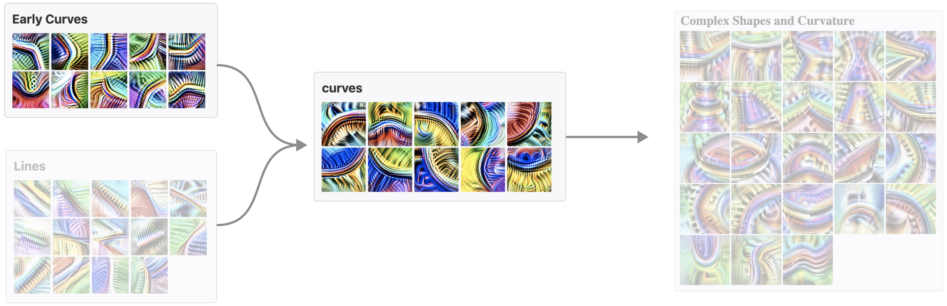
Each node marks a learned visual feature. Each arrow shows one feature feeding another. The induction circuit later in this lesson uses the same kind of account for tokens: name the features, trace the paths between them, and test whether those paths explain the behavior.
Curve circuit example from "Zoom In: An Introduction to Circuits" by Olah et al. (2020)
Slides: Introduction to mechanistic interpretability
Video: Introduction to mechanistic interpretability
Open the video in a new tab if the embedded player does not load.
Week 3 plan
Week 3 plan
- Read this page in order and run the two examples on it. Allow 45 to 60 minutes, and more if you stop to edit the code.
- Then open the 1.2 Introduction to Mechanistic Interpretability notebook in Colab and work through sections 1–2. Sections 3–4 are the next step, not required work for this session.
The induction problem
Suppose a model sees two copies of a short block of tokens:
Treat A, B, and C as stand-ins for arbitrary tokens, not a familiar phrase. The target under each chip is the usual next-token shift: logits at position i predict token i + 1. The final position has no supplied next-token target because the prompt ends there.
At the first A, nothing tells the model that B comes next. At the second A, the earlier transition A B is already in context. A model that can reuse that transition has a reason to predict the second B more confidently.
Repeated random blocks make a useful experiment. Randomness rules out memorizing a particular phrase. Repetition supplies a simple fact the model can recover from the prompt. If next-token loss reliably decreases on the second copy, the model is doing some form of in-context computation.
The mechanistic question for this lesson:
How does information about the first copy travel through the model and influence predictions on the second copy?
One proposed answer is induction: an early head records which token came before each position, and a later head uses that record to retrieve the continuation that followed the same token earlier. The proposal predicts a particular attention pattern we can look for.
Check yourself: observation or hypothesis?
“Loss decreases on the second half of many fresh repeated blocks” is an observation. “A previous-token head and induction head cause that improvement” is a hypothesis. If only the observation is known, what follows?
Answer: The model uses prompt information. Internal evidence is still needed to identify the mechanism.
TransformerLens: load, run, cache
We now have a reproducible behavior and a hypothesis about its mechanism. TransformerLens gives us named access points (hooks) for testing that hypothesis inside a model. A model's parameters are learned and persist across prompts. They include embedding matrices and attention weights: W_Q, W_K, and W_V form queries, keys, and values from the residual stream, and W_O writes each head's output back. Activations (residual vectors, queries, keys, values, attention patterns, and logits) are computed anew for each input.
HookedTransformer.from_pretrained loads both architecture and weights. to_tokens applies the model's tokenizer, while run_with_cache returns output logits and an ActivationCache of intermediate activations. remove_batch_dim=True strips the batch axis from the cached activations only; the returned logits keep theirs.
from transformer_lens import HookedTransformer
import circuitsvis as cv

model = HookedTransformer.from_pretrained("gpt2-small")
tokens = model.to_tokens("A short prompt")
logits, cache = model.run_with_cache(tokens, remove_batch_dim=True)
pattern = cache["pattern", 0]  # [head, destination, source]
resid = cache["resid_post", 0]  # [pos, d_model]

str_tokens = model.to_str_tokens(tokens[0])
print(list(enumerate(str_tokens)))
# [(0, '<|endoftext|>'), (1, 'A'), (2, ' short'), (3, ' prompt')]

print(tokens.shape, logits.shape, pattern.shape, resid.shape)
# torch.Size([1, 4]) torch.Size([1, 4, 50257]) torch.Size([12, 4, 4]) torch.Size([4, 768])

cv.attention.attention_patterns(tokens=str_tokens, attention=pattern)
Two indexing traps show up in that printout:
- GPT-2 tokens often carry the space before a word (
' short',' prompt'), so match token strings with their leading spaces. - TransformerLens prepends a beginning-of-sequence token (BOS) by default (
'<|endoftext|>'at position 0), so a short string often has more model positions than words.
BOS moves every absolute index by one. Relative offsets stay the same: "one position earlier" is still dest - 1.
The circuitsvis call plots the cached attention pattern with those token labels. Use it to see where a head reads.
These four shapes appear constantly:
| Object | Representative shape | Meaning |
|---|---|---|
| Tokens | [batch, pos] | Token IDs supplied to the model |
| Residual stream | [batch, pos, d_model] | Shared activation channel between layers |
| Attention pattern | [batch, head, dest, source] | Routing weights for each head |
| Logits | [batch, pos, d_vocab] | Scores for the next token |
Hook points do not all share the same axis order. Read .shape before you index, as in the snippet above.
Read an attention pattern
This is circuitsvis, the widget the Colab notebook draws when you call cv.attention.attention_patterns. It shows one destination-by-source grid per head. Hover a cell to read its exact weight; hover a token to see everything that position reads. Learn its look now. The notebook session uses it for every attention plot.
On this site we can also draw an attention matrix as a plain numbered grid. Same rows, same columns, same reading rule: cell (d, s) is pattern[d, s], how strongly destination d reads source s. The numbers appear inside the cells, so nothing hides behind a hover. The static grid below is an intentionally small schematic; the runnable cell later draws the real checkpoint values in this format. In Colab, its cv call draws a circuitsvis widget.
How to read the numbered grid:
- Find a destination token on the left.
- Move across its row to a source token at the top.
- Read the cell's attention weight. Darker cells carry more attention.
In this schematic, dark cells form a stripe two positions left of the diagonal. It is a hand-authored illustration of the reading rule, not a prediction of the exact cells the trained head will choose.
The grid is lower triangular because of causal attention. A destination can only read earlier positions and itself. The white upper-right triangle is the future, so information moves forward through the sequence. Each row sums to one.
That grid is only the routing step. One head starts from residual vectors X and builds three projections:
- queries
Q = XW_Q - keys
K = XW_K - values
V = XW_V
Query-key scores become the pattern you just read:
M is the causal mask. Softmax makes each destination row sum to one. That QK path answers where to read.
The head still has to write something back. It mixes the values with those weights, then maps into the residual stream:
That OV path answers what the read contributes. A stripe in circuitsvis shows routing. It does not show the content of the write.
Runs the real two-layer attention-only checkpoint on CPU. The cv call renders the reconstructed values as a numbered grid on this site and as circuitsvis in Colab.
import os
import torch as t
import circuitsvis as cv
from transformer_lens import HookedTransformer, HookedTransformerConfig

cfg = HookedTransformerConfig(
    d_model=768,
    d_head=64,
    n_heads=12,
    n_layers=2,
    n_ctx=2048,
    d_vocab=50278,
    attention_dir="causal",
    attn_only=True,
    tokenizer_name="EleutherAI/gpt-neox-20b",
    seed=398,
    use_attn_result=True,
    normalization_type=None,
    positional_embedding_type="shortformer",
)
model = HookedTransformer(cfg)
if "ARENA_MODEL_DIR" in os.environ:
    weights_path = os.path.join(os.environ["ARENA_MODEL_DIR"], "attn_only_2L_half.pth")
else:  # Colab: download the same checkpoint once.
    from huggingface_hub import hf_hub_download
    weights_path = hf_hub_download(
        "callummcdougall/attn_only_2L_half", "attn_only_2L_half.pth"
    )
model.load_state_dict(t.load(weights_path, map_location="cpu", weights_only=True))
model.eval()

# Change this to any prompt. Its text does not need to repeat or have a fixed length.
prompt = " A B C A B C"
tokens = model.to_tokens(prompt, prepend_bos=True)
# The course renderer accepts one head with at most 2,048 values, so display the
# first 45 model positions (45 × 45 = 2,025) when a prompt tokenizes longer.
if tokens.shape[1] > 45:
    print(f"Prompt has {tokens.shape[1]} positions; visualizing the first 45.")
    tokens = tokens[:, :45]
str_tokens = model.to_str_tokens(tokens[0])
_, cache = model.run_with_cache(tokens, remove_batch_dim=True)

layer, head = 1, 4  # L1H4 is an induction head in this trained checkpoint.
# With remove_batch_dim=True, q and k are [pos, head, d_head], while
# pattern is [head, destination, source]. Select one head without reordering pos.
q = cache["q", layer][:, head, :]
k = cache["k", layer][:, head, :]
cached_pattern = cache["pattern", layer][head]
assert q.shape == k.shape == (tokens.shape[1], model.cfg.d_head)

scores = q @ k.T / (model.cfg.d_head ** 0.5)
future = t.triu(t.ones_like(scores, dtype=t.bool), diagonal=1)
reconstructed = scores.masked_fill(future, -t.inf).softmax(dim=-1)

print("indexed tokens:", list(enumerate(str_tokens)))
print("q/k shape:", tuple(q.shape), "pattern shape:", tuple(cached_pattern.shape))
print("max |reconstructed - cached|:",
      (reconstructed - cached_pattern).abs().max().item())
print("row sums:", reconstructed.sum(dim=-1))
print("future mass:", reconstructed.triu(diagonal=1).sum().item())

cv.attention.attention_patterns(
    tokens=str_tokens,
    # circuitsvis expects [head, destination, source].
    attention=reconstructed.unsqueeze(0),
)
Induction heads: label, match, copy
A clean two-layer induction circuit does three things:
- A layer-0 previous-token head labels each position with its predecessor.
- A layer-1 induction head matches the current token against those labels and attends to the position after the earlier match.
- That same head copies continuation-related content toward the logits.
destination 3
A
layer 0 label @ src 1: follows A
reads src 1 → promotes B
destination 4
B
layer 0 label @ src 2: follows B
reads src 2 → promotes C
destination 5
C
layer 0 label @ src 3: follows C
reads src 3 → promotes A
no supplied next-token target
The label is a direction in the residual stream, not a literal string. Destination 3 reads source 1 (the B after the earlier A), because the useful continuation sits one position after the match.
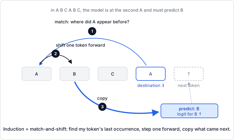
A, match the earlier A, shift to its continuation B, then promote B.This needs two layers. Heads in one layer run in parallel, so a head cannot read another same-layer head's new write. Layer 0 writes predecessor identity first. Layer 1 then reads that feature through its key path. That cross-layer use of an earlier head's output is K-composition.
For a repeated block of length N, the continuation source is
The stripe sits N - 1 cells left of the main diagonal. BOS shifts source and destination together, so the difference stays the same.
The offset follows from token matching and holds only while the second copy repeats the first. The builder below checks token identity: a destination whose token never appeared earlier has no source, and a token that appeared more than once earlier has more than one.
Quiz: build the induction circuit
Choose the predicting position. Find an earlier position with the same token, move one place right, and copy that continuation.
Try a counterexample or change the prompt
Input: choose the predicting destination
Predecessor to place: choose a token below, then choose its next position.
The final prompt position has no supplied next-token target, so its output cannot be scored.
Circuit terms: The predicting position is the destination. The earlier continuation is the source. The QK circuit chooses the source; the OV circuit copies its content. The earlier head's label reaches the later head's key through K-composition.
Find induction heads in the toy model
The toy model has 24 attention heads. We could inspect all 24 attention-pattern grids by eye, but we already know the clue we are looking for. On the second copy of a repeated block, an induction head should attend to the token that followed the earlier match. In the grid, those cells form an offset stripe.
circuitsvis draws each head's attention pattern as one of these grids: rows are destination tokens, columns are source tokens, and darker cells carry more attention. A few common patterns are worth recognizing:
| Motif | High cells | Signature |
|---|---|---|
| Previous token | source = dest - 1 | Stripe left of main diagonal |
| Current token | source = dest | Main diagonal |
| First token/BOS | source = 0 | Bright first column |
| Induction | source = dest - (N - 1) in copy two | Offset stripe in later rows |
Rather than eyeballing every grid, we can turn the induction stripe into one number. For each destination in the second copy, take the attention weight at its expected source, then average those weights. This is the induction score:
A score near 1 means the head places most of its attention on the expected induction cells. A score near 0 means it mostly looks elsewhere.
Why might my score differ from the notebook?
This page averages all N destinations in the second copy. A next-token version drops the final destination, which has no next-token target, and averages N - 1 cells instead.
The notebook uses pattern.diagonal(offset=1-seq_len) and averages every cell on that diagonal. With the BOS-prefixed sequence, that diagonal holds N + 2 cells: the N second-copy destinations plus two destinations from the first copy, whose values vary by head. The two conventions are therefore the notebook's full-diagonal mean over N + 2 cells and this page's mean over the N repeated positions. Scores and rankings can differ between them, so compare heads under the same definition on the same cache.
The example below creates a fresh repeated block, computes the score for every head, and selects the highest-scoring candidate. circuitsvis then draws that head's attention-pattern grid so you can check that the number corresponds to the stripe you expected.
Why use this toy checkpoint?
It has two layers with 12 heads each, but no MLPs or LayerNorm, so its attention circuits are unusually exposed. It also uses positional_embedding_type="shortformer": positional embeddings enter the key and query calculations, but not the values. The residual stream therefore cannot directly carry position, and induction heads form two to three times earlier in training.
Example 2: find an induction head in the toy checkpoint
Edit and run this PyTorch example. The toy checkpoint is already cached on the course CPU, so no download happens here.
import os
import torch as t
import circuitsvis as cv
from transformer_lens import HookedTransformer, HookedTransformerConfig

cfg = HookedTransformerConfig(
    d_model=768,
    d_head=64,
    n_heads=12,
    n_layers=2,
    n_ctx=2048,
    d_vocab=50278,
    attention_dir="causal",
    attn_only=True,
    tokenizer_name="EleutherAI/gpt-neox-20b",
    seed=398,
    use_attn_result=True,
    normalization_type=None,
    positional_embedding_type="shortformer",
)
model = HookedTransformer(cfg)
# ARENA_MODEL_DIR is this site's pre-populated model cache. In Colab, use
# hf_hub_download("callummcdougall/attn_only_2L_half", "attn_only_2L_half.pth") instead.
weights_path = os.path.join(
    os.environ["ARENA_MODEL_DIR"],
    "attn_only_2L_half.pth",
)
model.load_state_dict(t.load(weights_path, map_location="cpu", weights_only=True))
model.eval()

t.manual_seed(0)
N = 20
bos = t.tensor([[model.tokenizer.bos_token_id]], device=model.cfg.device)
block = t.randint(0, model.cfg.d_vocab, (1, N), device=model.cfg.device)
tokens = t.cat([bos, block, block], dim=1)
_, cache = model.run_with_cache(tokens, remove_batch_dim=True)

# BOS-prefixed indexing: second copy is destinations N+1 ... 2N.
dest = t.arange(N + 1, 2 * N + 1, device=model.cfg.device)
source = dest - (N - 1)
scores = t.stack([
    cache["pattern", layer][:, dest, source].mean(-1)
    for layer in range(model.cfg.n_layers)
])
layer, head = divmod(scores.argmax().item(), model.cfg.n_heads)
print(f"Best candidate: L{layer}H{head}, score={scores[layer, head]:.3f}")
cv.attention.attention_patterns(
    tokens=model.to_str_tokens(tokens[0]),
    attention=cache["pattern", layer][head:head+1],
)
In this checkpoint, heads 1.4 and 1.10 usually have strong induction scores, while 0.7 is a prominent previous-token head. Rerun the search with different random blocks and block lengths, then try a shuffled or nonrepeated second half. A genuine induction pattern should be stable across repeated blocks and weaken when the repetition is broken.
The label describes what a head does on a particular input, not what it must do on every prompt. For example, 1.4 can look like an induction head on repeated tokens and a first-token head on ordinary prose. And even a consistently high induction score only establishes a routing pattern; it does not yet show that the head's OV write improves the prediction or that the head is causally necessary.
Video: Finding a circuit with the Transformer Explainer
This walkthrough returns to the Transformer Explainer site from week 2 and tries to find a circuit.
Open the video in a new tab if the embedded player does not load.
Notebook session
Open the [1.2] Intro to Mech Interp notebook and focus on sections 1–2:
- load GPT-2 Small; inspect tokenization, BOS, config, parameters, logits, and cached activations
- read
cache["pattern", layer]and visualize labeled heads with circuitsvis - load the attention-only checkpoint and compare first-copy with second-copy loss
- identify four attention motifs, implement induction scores, and check scores against plots and controls
You are done when you can align each input with its next-token label, explain a cell as “destination reads source,” derive the N - 1 offset, and separate a behavioral observation from a mechanistic hypothesis.
Later in the notebook. Sections 3–4 introduce hooks, ablation, direct logit attribution, and reverse-engineering QK/OV circuits. A stripe shows routing. Exact-token induction covers only one kind of in-context learning. Treat those sections as the next step, not required work for this session.
Quiz
review quiz
Further reading
this week's practice
core
- Complete sections 1–2 of the 1.2 notebook
stretch
- Continue into sections 3–4: hooks, ablation, direct logit attribution, and QK/OV circuits