week 01 / 12
Orientation and a first digit classifier
Follow one MNIST digit through tensors, an MLP, and a training step.
companion notebook · ARENA 0.2, sections 1 and 2
Use after the prework below.
new terms this week · 22
Tensor concepts
Tensor operations
- Broadcasting
- PyTorch automatically expands compatible smaller tensors across missing dimensions before an operation.
- einops
- A small library for readable tensor rearrangement, reduction, and repetition.
- einsum
- Index-notation syntax for dot products, matrix multiplies, reductions, and many tensor contractions.
Parameters & layers
- Weight
- A learnable number inside a model, usually stored in a tensor.
- Bias
- A learnable offset added after a weighted sum.
- ReLU
- The function max(0, x). It lets stacked layers represent more than one linear operation.
- Residual connection
- A direct branch that adds an earlier activation to the output of other layers: out = x + f(x).
- Batch normalization
- A layer that normalizes each channel during training, then applies a learned scale and offset.
- Convolution
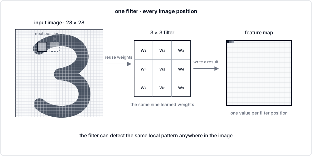
- An operation that applies the same small kernel at each position in an image to find local patterns.
Outputs & objectives
- Logits
- Raw model scores before softmax converts them into probabilities.
- Softmax
- A function that turns a vector of scores into a probability distribution by exponentiating and normalising.
- Cross-entropy
- The standard classification loss. It measures how little probability the model put on the correct label.
Optimization
- Gradient
- For each parameter, the gradient describes how a small increase would change the loss.
- SGD
- Stochastic gradient descent: step parameters opposite the gradient.
- Learning rate
- The step size an optimizer uses when updating parameters.
- Adam
- A popular optimizer that adapts per-parameter step sizes using running gradient statistics.
Training controls
- Weight decay
- A regularizer that nudges weights toward zero during optimization, discouraging solutions that require large parameter values.
Automatic differentiation
- Chain rule
- The rule that lets backprop multiply local derivatives through a composed computation.
- Computational graph
- A graph of tensor operations whose reverse traversal computes gradients.
- Autograd
- Automatic differentiation: software that builds and backpropagates through a computation graph.
This week is our foundation, and we are going from tensors all the way to backpropagation, building the core mental model that supports everything else in the course.
The reason we start here is that tensors are the basic data structure underneath almost everything we will do, including images, activations, gradients, and the data flowing through models. If you get comfortable reading shapes and understanding what each axis means, the rest of the course becomes much easier.
Over the next sections, we will move from tensor basics, to some PyTorch practice with rays, to building and training a simple model, and then into optimization and backpropagation. The goal is not to rush ahead, but to build intuition step by step so these ideas feel solid when we see them again later.
Slides: Foundations through one digit classifier
Week 1 plan
Week 1 plan
- Read this page in order. Run the code cells and feel free to modify them. Allow 60 to 75 minutes.
- In the warm-up you practice tensor operations with small examples you can run in the browser.
- Then you follow one handwritten digit through a model and its five training operations.
- Finally, open the 0.2 CNNs & ResNets notebook to implement the model, train it, and check its accuracy.
Warm up with tensors and a simple ray example
What is a tensor?
A tensor is a multidimensional array of numbers. Its shape lists the size of each axis and helps you identify the data it holds.
| Shape | Name |
|---|---|
() | scalar |
(n,) | vector |
(m, n) | matrix |
(H, W) | image |
(B, H, W) | batch of images |
Warm up with one tiny image
The warm-up builds toward two bigger examples: rays, the lines a camera casts through an image plane in ray tracing, and MNIST, a dataset of handwritten digits. Before those, start with a tiny 2 by 3 grayscale image. This tensor has a height axis with two rows and a width axis with three columns.
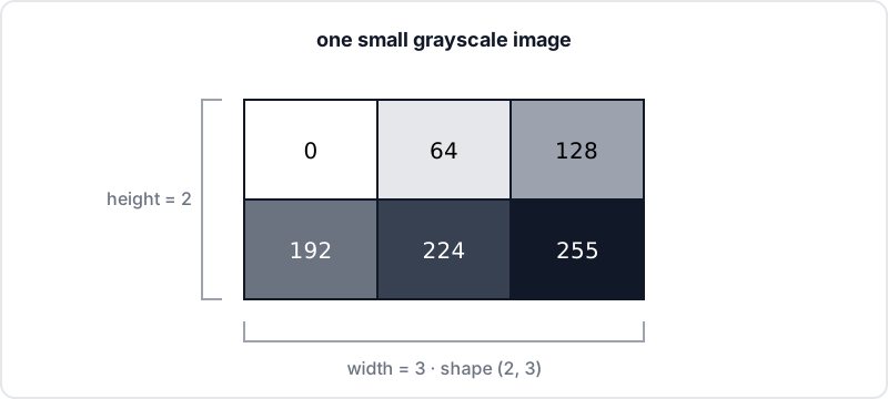
A shape records the size of each axis. Here, (2, 3) means two rows and three columns.
Edit the code, then run it on the course CPU.
import torch

image = torch.tensor([[0, 64, 128], [192, 224, 255]], dtype=torch.float32)
print(image.shape, image.dtype)
print(image[0])       # first row; indexing removes the height axis
print(image[:, 1:])  # every row, last two columns
# torch.Size([2, 3]) torch.float32
# tensor([  0.,  64., 128.])
# tensor([[ 64., 128.], [224., 255.]])
dtype names the kind of value stored in the tensor. float32 stores floating point numbers. The colon in a slice means "take every position" on that axis.
Suppose you want to brighten the image by adding 32 to every pixel. In plain Python, you could use one loop over the rows and another over the columns. PyTorch applies one operation to every selected value at once. This is a vectorized operation. It avoids one Python step per pixel and is faster on large tensors.
Edit the code, then run it on the course CPU.
import torch

image = torch.tensor([[0, 64, 128], [192, 224, 255]], dtype=torch.float32)
brighter = (image + 32).clamp(max=255)
print(brighter)
# tensor([[ 32.,  96., 160.],
#         [224., 255., 255.]])
The addition acts on all six pixels at once. clamp caps every value at 255, the largest valid brightness. Without it, the two brightest pixels would land above 255. The shape stays (2, 3).
Cast rays through a pixel grid
In this course, ray tracing is practice with tensors. You cast one ray per pixel and find a point along each ray. ARENA's full exercise builds a renderer, a program that turns a 3D scene into a 2D image. You do not need that this week, only the shape skills.
A ray starts at an origin O and follows a direction D. The value t controls how far the point moves along D:
point = O + t · D
One camera ray passes through each image pixel. A grid of pixels needs a grid of directions. With two rows and three columns, directions.shape == (2, 3, 3): height, width, and three coordinates named xyz.
Scroll the diagram sideways on a small screen.
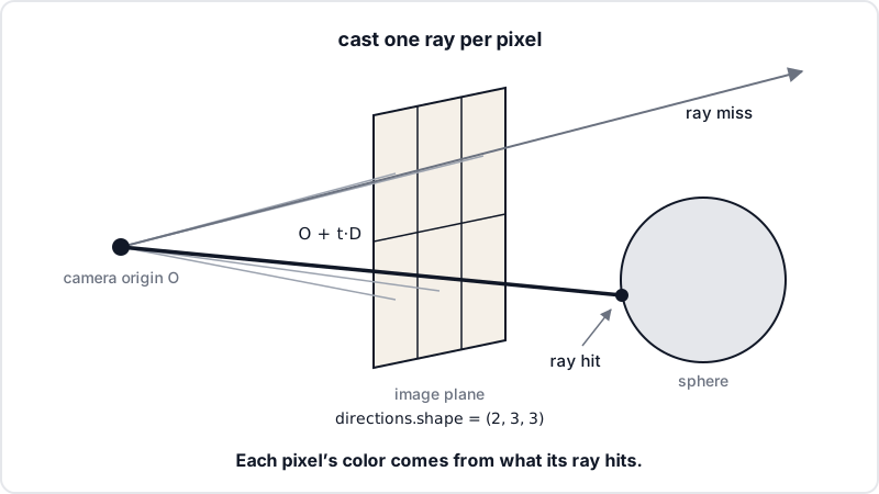
The image axes select a ray. The final axis stores its x, y, and z direction.
Edit the code, then run it on the course CPU.
import torch

origin = torch.tensor([0.0, 0.0, 0.0])
directions = torch.tensor([
    [[1, -1, -1], [1, -1, 0], [1, -1, 1]],
    [[1,  1, -1], [1,  1, 0], [1,  1, 1]],
], dtype=torch.float32)
points = origin + 2.0 * directions
print(points.shape, points[0, 1])
# torch.Size([2, 3, 3]) tensor([ 2., -2.,  0.])
Look at the shapes in that sum. origin is (3,) and directions is (2, 3, 3). PyTorch broadcasts the smaller tensor. It reuses the same three origin coordinates for every ray, so you do not have to write a loop or copy the origin six times. Check the shapes before you run the code. When an operation fails, the error message often shows which shapes do not match.
To build the full renderer, work through the 0.1 Ray Tracing notebook.
Name the axes
Einstein notation gives tensor axes short names. Once the axes have names, one pattern string can describe a transpose, a sum, or a matrix multiplication. You stop memorizing a separate function for each operation and instead write which axes go in and which axes come out.
Start with the tiny image from the warm-up and name its two axes h and w. The pattern "hw->wh" says the image goes in with height first and comes out with width first. That is a transpose.
The -> arrow separates input axes from output axes. Two rules cover every pattern:
- An axis named after the
->survives into the result, in the order written there. - An axis missing after the
->is summed away.
So "hw->h" sums along width and leaves one total per row, and "hw->" sums away both axes and leaves one number.
Edit the code, then run it on the course CPU.
import torch

image = torch.tensor([[0, 64, 128], [192, 224, 255]], dtype=torch.float32)
print(torch.einsum("hw->wh", image).shape)  # transpose
print(torch.einsum("hw->h", image))         # sum along width
print(torch.einsum("hw->", image))          # sum everything
# torch.Size([3, 2])
# tensor([192., 671.])
# tensor(863.)
With two inputs there is one more rule. An axis named in both inputs lines up matching values for multiplication. The pattern "hw,w->h" uses every rule at once. w is named in both inputs, so each image value multiplies its matching weight. w is missing after the ->, so the products sum. h survives, so a (2, 3) image and (3,) weights give (2,) row scores.
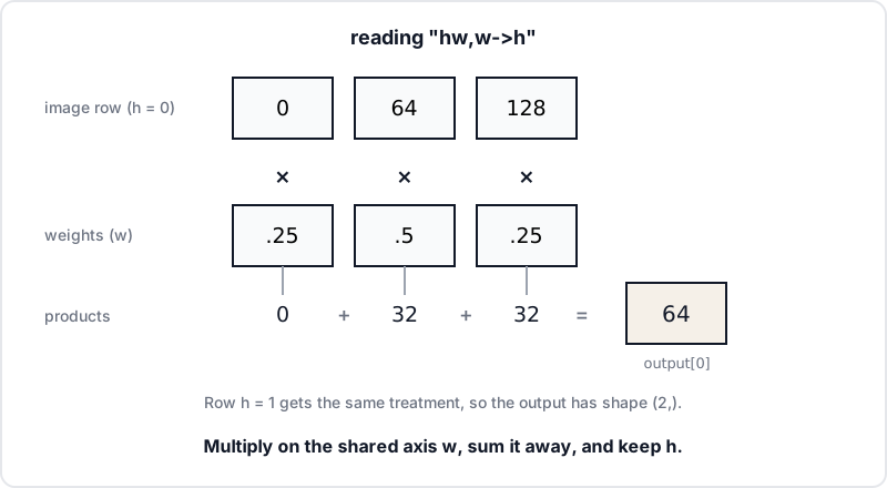
This weighted sum along one axis is the same pattern the Linear layer uses later on this page.
For the ray grid, use h for height, w for width, and x for the three coordinates in each direction vector. On directions with shape (h, w, x), the h and w axes pick a ray. The x axis stores the three direction components.
Write it with einsum
einsum is Einstein notation you can run. The pattern string lists the axis names for each input, separated by commas, then the output axes after the ->.
In "hwx,->hwx", the first input has axes h, w, and x. The second input is the scalar t, which has no axes, so its slot before the -> is empty. Every named axis remains in the output. The operation multiplies each direction component by t without summing any axis.
Edit the code, then run it on the course CPU.
import torch

directions = torch.tensor([
    [[1, -1, -1], [1, -1, 0], [1, -1, 1]],
    [[1,  1, -1], [1,  1,  0], [1,  1,  1]],
], dtype=torch.float32)
t = torch.tensor(2.0)
scaled = torch.einsum("hwx,->hwx", directions, t)
print(scaled.shape, scaled[0, 1])
# torch.Size([2, 3, 3]) tensor([ 2., -2.,  0.])
ARENA also uses einops.einsum, where the same pattern can use full names: einsum(directions, t, "height width x, -> height width x").
Redo the ray step with einsum
The broadcast version wrote points = origin + 2.0 * directions. The einsum version names the scale step, then adds the origin.
Edit the code, then run it on the course CPU.
import torch

origin = torch.tensor([0.0, 0.0, 0.0])
directions = torch.tensor([
    [[1, -1, -1], [1, -1, 0], [1, -1, 1]],
    [[1,  1, -1], [1,  1,  0], [1,  1,  1]],
], dtype=torch.float32)
t = torch.tensor(2.0)
scaled = torch.einsum("hwx,->hwx", directions, t)
points = origin + scaled
print(points.shape, points[0, 1])
# torch.Size([2, 3, 3]) tensor([ 2., -2.,  0.])
You should see the same shape and point as in the broadcasting cell. Einsum expresses the same computation with named axes. The Linear layer in the next section uses the same axis rules with different names.
Follow one digit through the model
Meet MNIST
MNIST contains 70,000 handwritten digits. Each digit is a 28 by 28 grayscale image labeled from 0 to 9.
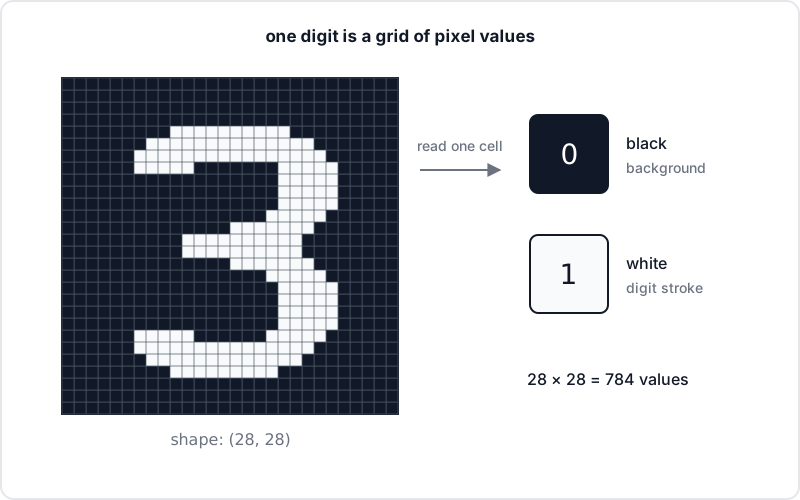
After the notebook converts an image to a float tensor, each pixel has a value from 0 to 1. Here, 0 is black and 1 is white. The notebook then normalizes each pixel with Normalize((0.1307,), (0.3081,)), which computes (x - 0.1307) / 0.3081. The model inputs therefore range from about −0.424 to 2.821. The model receives 784 separate pixel values and learns which patterns identify each digit.
The Week 1 model
You train a small neural network to recognize handwritten digits from MNIST.
The model receives one image with this shape:
Runs on the course CPU runner.
import torch

image = torch.zeros((1, 1, 28, 28))
print(image.shape)
print(image.shape == (1, 1, 28, 28))
# torch.Size([1, 1, 28, 28])
# True
The model produces ten logits. Each logit is a score for one digit from 0 to 9. Training changes the model's weights so that the correct digit tends to have the largest score.
The model runs this computation:
Scroll the diagram sideways on a small screen.
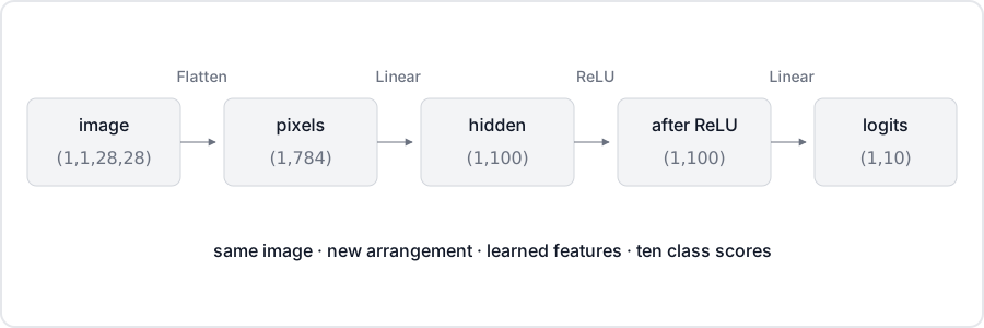
Keep the batch axis and follow the other axes from pixels to class scores.
The core work uses Sections 1 and 2 of 0.2 CNNs & ResNets. Convolutions and ResNets are stretch work.
Name the MNIST axes
An MNIST input adds batch and channel axes on top of height and width:
| Axis | Size | Meaning |
|---|---|---|
| batch | 1 | The model is processing one image. |
| channel | 1 | The image is grayscale. |
| height | 28 | The image has 28 rows of pixels. |
| width | 28 | The image has 28 columns of pixels. |
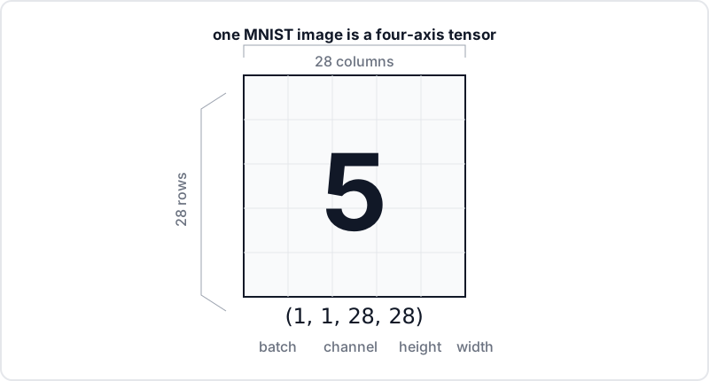
The first 1 means one image in the batch. The second 1 means one grayscale channel.
Edit the code, then run it on the course CPU.
shape = (1, 1, 28, 28)
batch, channels, height, width = shape

print("batch:", batch)
print("channels:", channels)
print("height:", height)
print("width:", width)
print("one image channel:", (height, width))
You should see the four axis sizes followed by one image channel: (28, 28).
What is the shape of a training batch?
With a batch size of 64, the shape is (64, 1, 28, 28). Only the batch axis changes. Each image still has one channel, 28 rows, and 28 columns.
Rearrange the pixels with Flatten
The first model operation is Flatten. It combines the channel, height, and width axes into one feature axis:
(1, 1, 28, 28) → (1, 784)
There are 1 × 28 × 28 = 784 pixel values. Flatten only rearranges them. No value is removed, added, or changed.
Edit the code, then run it on the course CPU.
batch, channels, height, width = 1, 1, 28, 28
features = channels * height * width

print((batch, features))
# (1, 784)
In the live notebook, ARENA supplies a Flatten module. Your SimpleMLP will use it before the first linear layer.
Turn pixels into hidden values
A linear layer has learned weight values and a learned bias. The first layer receives 784 pixel values and produces 100 hidden values:
Runs on the course CPU runner.
import torch

pixels = torch.zeros((1, 784))
weight = torch.zeros((100, 784))
bias = torch.zeros((100,))
hidden = pixels @ weight.T + bias

print("pixels:", pixels.shape)
print("weight:", weight.shape)
print("bias:", bias.shape)
print("hidden:", hidden.shape)
Each hidden value uses one row of 784 weights. The layer multiplies each pixel by its matching weight, adds the 784 products, and then adds one bias value. That is the weighted sum from the einsum diagram, with 784 positions instead of 3.
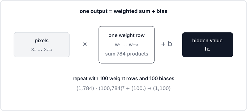
einsum uses the same axis rules as the ray warm-up, now with the full axis names from ARENA's Linear solution:
Runs on the course CPU runner.
import torch
from einops import einsum

pixels = torch.ones((1, 784))
weight = torch.ones((100, 784))
bias = torch.zeros((100,))

hidden = einsum(
    pixels,
    weight,
    "batch in_features, out_features in_features -> batch out_features",
)
hidden = hidden + bias

print(hidden.shape)
print(hidden[0, 0])
# torch.Size([1, 100])
# tensor(784.)
The pattern follows three rules:
batchremains because each image needs its own result.out_featuresremains because the layer produces 100 hidden values.in_featuresappears in both inputs but not the output, so the layer sums over all 784 input values.
Edit the code, then run it on the course CPU.
import torch

inputs = torch.tensor([[2, 1, -1, 3]], dtype=torch.float32)
weight = torch.tensor([
    [ 1, 0, 1, 0],
    [ 0, 2, 0, 1],
    [-1, 0, 1, 1],
], dtype=torch.float32)
bias = torch.tensor([1, -1, 2], dtype=torch.float32)

outputs = torch.einsum("bi,oi->bo", inputs, weight) + bias
print(outputs)
# tensor([[2., 4., 2.]])
Why does the input feature axis disappear?
The operation multiplies matching input and weight values, then adds across all input features. One value remains for each image and output feature.
Apply ReLU between the linear layers
ReLU follows the first linear layer. It replaces each negative value with zero and leaves each positive value unchanged:
Edit the code, then run it on the course CPU.
def relu(x):
    return max(x, 0.0)

hidden = [-3.0, -0.5, 0.0, 1.5, 4.0]
after_relu = [relu(value) for value in hidden]

print(after_relu)
# [0.0, 0.0, 0.0, 1.5, 4.0]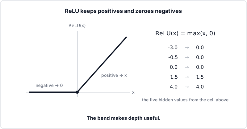
Without ReLU, two linear layers in a row have the same effect as one linear layer. ReLU changes the values between the layers, so the full model can represent functions that one linear layer cannot.
Runs on the course CPU runner.
import torch
from torch import nn

class SimpleMLP(nn.Module):
    def __init__(self):
        super().__init__()
        self.flatten = nn.Flatten()
        self.linear1 = nn.Linear(28 * 28, 100)
        self.relu = nn.ReLU()
        self.linear2 = nn.Linear(100, 10)

    def forward(self, x):
        x = self.flatten(x)
        x = self.linear1(x)
        x = self.relu(x)
        return self.linear2(x)


model = SimpleMLP()
image = torch.zeros((1, 1, 28, 28))
logits = model(image)
print(logits.shape)
# torch.Size([1, 10])
This runnable version uses PyTorch's layers. In the first core exercise, you implement the same structure with the notebook's own Flatten, Linear, and ReLU classes. The notebook supplies Flatten, but leaves ReLU and Linear unimplemented, with working answers in solution dropdowns. Before you start SimpleMLP, copy and run the ReLU and Linear solutions, then run the Flatten cell.
Choose the largest logit
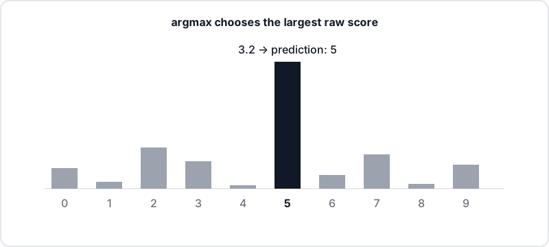
The final layer returns a tensor with shape (1, 10). These ten values are logits. A logit is a raw score for one digit class.
Edit the code, then run it on the course CPU.
import torch

logits = torch.tensor([[0.2, -0.4, 1.1, 0.6, -0.8, 3.2, 0.0, 0.9, -0.2, 0.3]])
prediction = logits.argmax().item()

print(prediction)
# 5
argmax returns the index of the largest logit. The largest value is 3.2 at index 5, so the predicted digit is 5.
Softmax turns logits into probabilities that add to 1. During training, pass the raw logits to cross-entropy. F.cross_entropy computes the loss directly from those logits, so do not apply softmax first.
Run the five-step training loop
Send the loss backward
The forward pass pushes one digit through Flatten, two linear layers, ReLU, and cross entropy to produce a single loss value. While it does this, PyTorch records the operations it needs to differentiate the loss with respect to the trainable parameters in a computational graph. The graph stores which tensors produced each result. The input image does not require gradients, so PyTorch does not compute a gradient for the image.
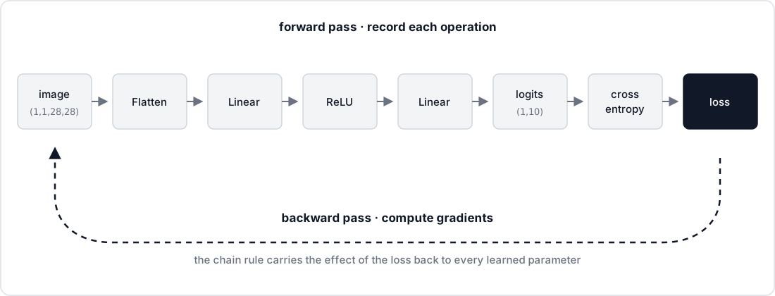
The forward pass builds the graph from left to right. Backpropagation follows it from right to left.
When you call loss.backward(), PyTorch follows the graph from the loss back to every weight and bias and computes a gradient for each one.
A gradient answers one local question. If this parameter increased by a very small amount, how would the loss change? The optimizer uses that answer in step 4, the parameter update.
You do not need to implement backpropagation yourself this week. The 0.4 Backpropagation notebook is stretch work.
Repeat five operations to learn
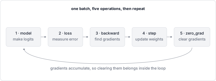
One training step has five operations:
Scroll the diagram sideways on a small screen.
Runs on the course CPU runner.
import torch
from torch import nn
from torch.nn import functional as F

torch.manual_seed(0)
model = nn.Sequential(
    nn.Flatten(),
    nn.Linear(28 * 28, 100),
    nn.ReLU(),
    nn.Linear(100, 10),
)
optimizer = torch.optim.SGD(model.parameters(), lr=0.01)
images = torch.rand((4, 1, 28, 28))
labels = torch.tensor([0, 1, 2, 3])

logits = model(images)                  # 1. run the model
loss = F.cross_entropy(logits, labels) # 2. measure the loss
loss.backward()                        # 3. compute gradients
optimizer.step()                       # 4. update parameters
optimizer.zero_grad()                  # 5. clear gradients

print("logits shape:", logits.shape)
print("loss:", round(loss.item(), 4))
This example uses four random images. The notebook supplies real MNIST images and labels.
The SGD optimizer in this cell uses the plain gradient descent update:
θ ← θ − η · g
θ represents the current parameters. g is the gradient from loss.backward(). η is the learning rate, the step size.
Here, optimizer.step() applies that update. Other optimizers, such as momentum and Adam/AdamW, transform the gradient before the step, and some add weight decay. PyTorch adds new gradients to the gradients already stored on each parameter. optimizer.zero_grad() clears them before the next batch. Without step 5, the next update would use gradients from more than one batch.
Optimizer types
Different optimizers use the gradient in different ways. A loss surface plots parameter values against the resulting loss.
| Optimizer | What it does |
|---|---|
| SGD | Uses the current gradient |
| Momentum | Uses current and past gradients to reduce changes in direction |
| RMSProp | Adjusts the step size for each parameter using recent gradients |
| Adam / AdamW | Combines momentum with a separate step size for each parameter; AdamW is the usual default |
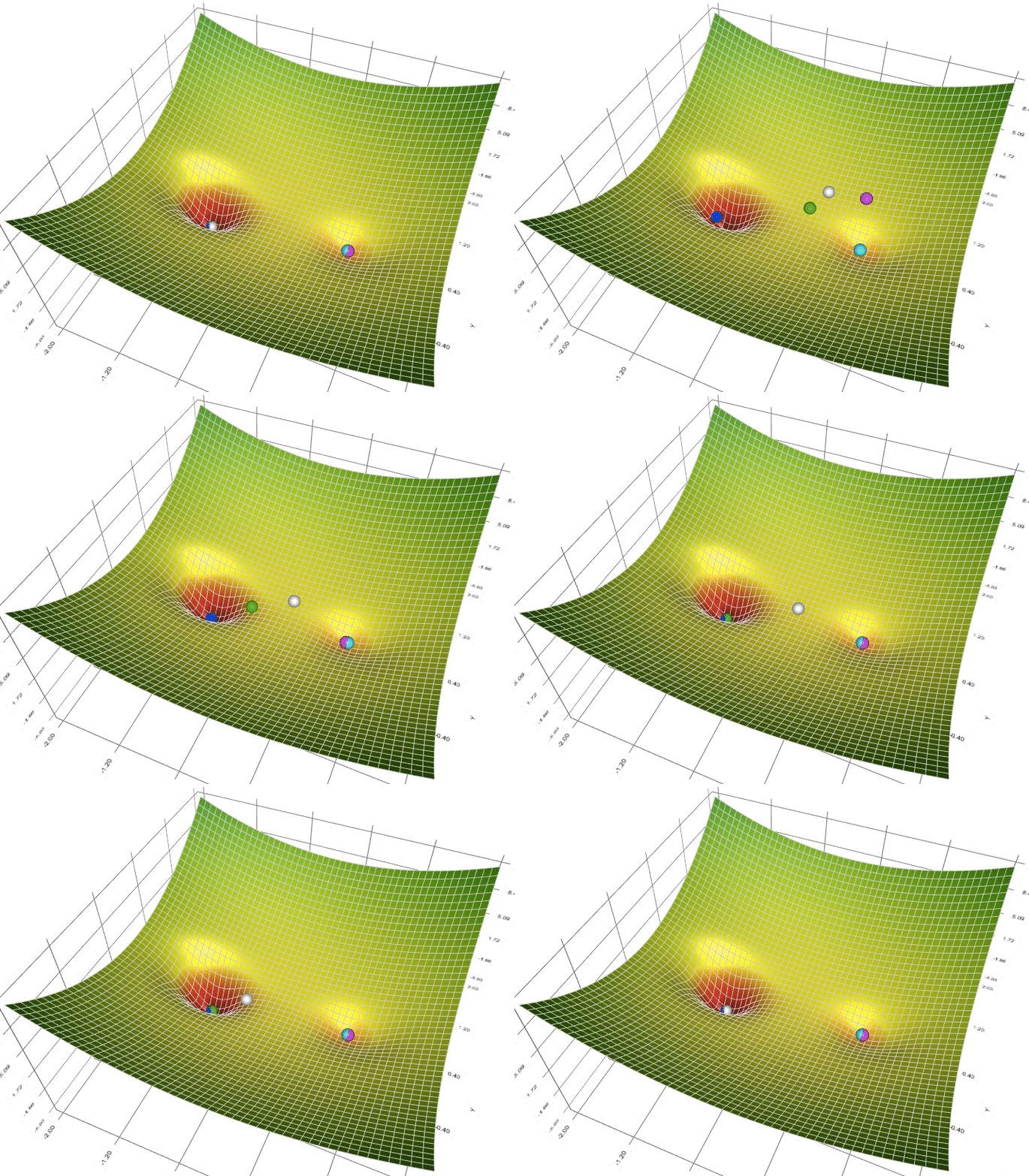
The name colors match the balls: SGD is cyan, Momentum is magenta, RMSProp is green, and Adam is blue. AdaGrad is white. Each optimizer follows a different path across the same loss surface. SGD zigzags, while Momentum overshoots. RMSProp and Adam adjust their steps across steep and flat directions. No optimizer wins everywhere. The learning rate still affects every path.
The runnable cell above uses SGD. That is enough for the notebook this week. 0.3 Optimization is where you write these update rules and sweep the settings.
Check progress on held-out images
Training loss tells you how the model performed on the batches used to update it. You also need images that were held back from training.
The notebook uses its test set for validation. The validation loop follows four steps:
- Run the model inside
torch.inference_mode()because validation needs no gradients. - Take
argmax, the index of the largest of the ten logits, to get one predicted digit per image. - Compare the predictions with the true labels.
- Divide the number of correct predictions by the number of test images.
The model changes after every training batch, so the notebook records training loss for every batch. The model does not change during validation, so the notebook records one validation accuracy after each epoch, one full pass through the training set.
The second core exercise asks you to add this validation loop to the supplied train function.
Look ahead to image-aware models
SimpleMLP flattens the image before it learns. Flatten keeps the pixel order and can be reversed, so no information is lost. The fully connected model does not build in local connectivity or shared image filters.
A convolution keeps the image axes intact. It applies the same small set of weights at every position in the image.
A ResNet stacks residual blocks, groups of convolutional layers with a direct path around them. In the simplified block below, two 3 by 3 convolutions with a ReLU between them compute an update F(x) with the same shape as x. A skip connection, a direct path around the convolutions, carries x to the end. The block adds x and F(x), then applies ReLU:
output = ReLU(x + F(x))
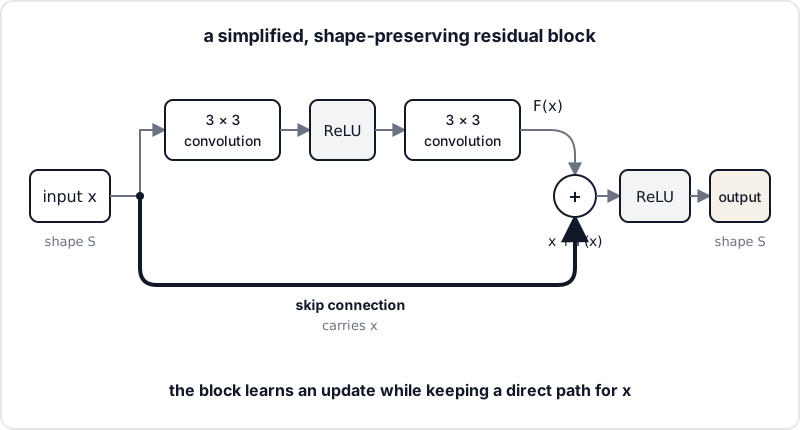
The skip connection gives information and gradients a direct path through the block. This makes deeper networks easier to train.
The full block in the notebook also applies batch normalization after each convolution to normalize and rescale each channel during training.
The training loop you use this week is the same one you will use for convolutions and ResNets. The shapes change. The five training steps stay the same.
Results checklist
The core notebook path starts at Simple Multi Layer Perceptron in Section 1 and stops after add a validation loop in Section 2. First copy and run the ReLU and Linear solutions and run the Flatten cell, so SimpleMLP does not hit a NotImplementedError.
You will complete two exercises:
- Implement
SimpleMLPand passtests.test_mlp_moduleandtests.test_mlp_forward. - Add a validation loop that records one accuracy value after each epoch.
When the notebook works:
- The training loss falls over three epochs.
- Test accuracy is above 80 percent after the first epoch, the figure ARENA gives.
- Test accuracy stays well above chance (10 percent) and improves across epochs.
Five checks before the notebook
You are ready when you can answer these without looking back:
- What does each axis in
(1, 1, 28, 28)mean? - Why does
Flattenproduce 784 values for each image? - Why is
in_featuresmissing from the einsum output? - Why should
F.cross_entropyreceive raw logits? - What are the five operations in one training step?
Show all answers
- The axes are batch, grayscale channel, height, and width.
- One image has
1 × 28 × 28 = 784pixel values. Flatten combines those three axes and keeps the batch axis. - The linear layer multiplies and sums across all input features, so that axis does not remain.
F.cross_entropycomputes the loss directly from raw logits. Applying softmax first gives it the wrong input.- Run the model, compute the loss, call
backward(), callstep(), and clear the gradients.
Stretch work
Complete stretch work only after the required prework and core exercises.
- Implement
ReLUandLinearin 0.2 CNNs & ResNets without using the supplied checkpoint answers. - Complete Section 3 on convolutions.
- Complete Section 4 on ResNets.
- Use 0.0 Prerequisites for more tensor and einsum practice.
- Use 0.3 Optimization to implement optimizers and sweep hyperparameters.
- Use 0.4 Backpropagation to build a small automatic differentiation system.
- Use 0.1 Ray Tracing for the full renderer.
- Complete 0.5 VAEs & GANs after the other Chapter 0 work.